Europe built parental leave for mothers first

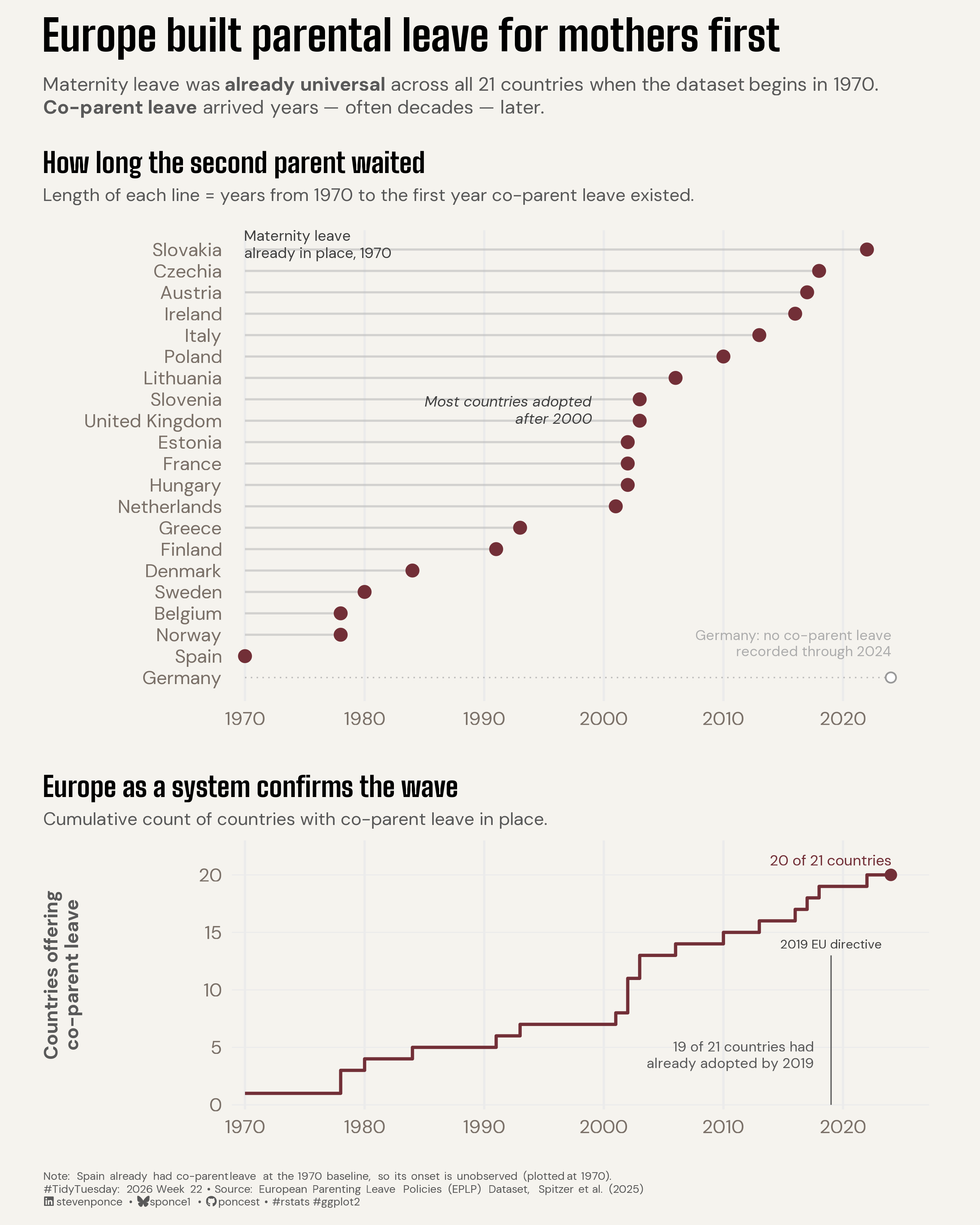
Maternity leave was already universal across all 21 countries when the dataset begins in 1970. Co-parent leave arrived years — often decades — later.

Across 21 European countries, maternity leave was universal by 1970 but co-parent leave arrived decades later — most after 2000, and Germany not at all. A two-panel lollipop and cumulative step chart trace adoption at the country and system scale. Built in R with ggplot2 and patchwork.

Figure 1: A two-panel chart titled “Europe built parental leave for mothers first,” covering 21 European countries from 1970 to 2024. The top lollipop panel shows each country’s first year of co-parent leave: maternity leave was already universal in 1970, but co-parent leave came far later — Spain already had it in 1970, most countries adopted only after 2000 (median 2002), and Germany had none through 2024. The bottom step panel shows the cumulative number of countries offering co-parent leave rising to 20 of 21, with a note that 19 of 21 had already adopted before the 2019 EU work-life balance directive. Together, the panels reveal that Europe established maternity leave first and extended leave to co-parents decades later. Source: European Parenting Leave Policies (EPLP) Dataset, Spitzer et al. (2025).

Steps to Create this Graphic

1. Load Packages & Setup

```{r}
#| label: load
#| warning: false
#| message: false      
#| results: "hide"     

## 1. LOAD PACKAGES & SETUP ----
suppressPackageStartupMessages({
if (!require("pacman")) install.packages("pacman")
pacman::p_load(
    tidyverse, ggtext, showtext, janitor, ggrepel,      
    scales, glue, skimr, patchwork, countrycode
    )
})

### |- figure size ----
camcorder::gg_record(
  dir    = here::here("temp_plots"),
  device = "png",
  width  = 8,
  height = 10,
  units  = "in",
  dpi    = 320
)

# Source utility functions
suppressMessages(source(here::here("R/utils/fonts.R")))
source(here::here("R/utils/social_icons.R"))
source(here::here("R/utils/image_utils.R"))
source(here::here("R/themes/base_theme.R"))
```

2. Read in the Data

```{r}
#| label: read
#| include: true
#| eval: true
#| warning: false

tt <- tidytuesdayR::tt_load(2026, week = 22)
eplp_raw <- tt$eplp |> clean_names()
rm(tt)
```

3. Examine the Data

```{r}
#| label: examine
#| include: true
#| eval: true
#| results: 'hide'
#| warning: false

glimpse(eplp_raw)
```

4. Tidy Data

```{r}
#| label: tidy
#| warning: false

### |- sentinel cleanup ----
## -98 (numeric) and "Not applicable" (character) are NOT zeros — recode to NA.
## co_ld == 0 is a REAL value (no co-parent leave) and must survive untouched;
## na_if(x, -98) leaves 0 alone by construction.
eplp <- eplp_raw |>
  mutate(
    across(where(is.numeric), \(x) na_if(x, -98)),
    across(where(is.character), \(x) na_if(x, "Not applicable"))
  )

### |- country code ----
## EU datasets often use UK/EL rather than ISO-2 GB/GR
eplp <- eplp |>
  mutate(
    country = recode(country, "UK" = "GB", "EL" = "GR"),
    country_name = countrycode(country, origin = "iso2c", destination = "country.name")
  )

baseline_year <- min(eplp$year, na.rm = TRUE)
max_year <- max(eplp$year, na.rm = TRUE)

mat_at_baseline <- eplp |>
  filter(year == baseline_year) |>
  mutate(has_maternity = (coalesce(mat_m_ld_ab, 0) > 0 |
    coalesce(mat_v_ld_ab, 0) > 0 |
    coalesce(mat_m_ld_bb, 0) > 0 |
    coalesce(mat_v_ld_bb, 0) > 0)) |>
  summarise(n_with_maternity = sum(has_maternity), n_total = n())

### |- co-parent leave adoption year (first year co_ld > 0) ----
adoption <- eplp |>
  filter(co_ld > 0) |>
  summarise(adopt_year = min(year), .by = country_name)

### |- Panel A data: waiting-time per country ----
panel_a <- eplp |>
  distinct(country_name) |>
  left_join(adoption, by = "country_name") |>
  mutate(
    adopted = !is.na(adopt_year),
    end_x = if_else(adopted, adopt_year, max_year),
    wait = end_x - baseline_year
  ) |>
  arrange(adopted, desc(adopt_year)) |>
  mutate(country_name = fct_inorder(country_name))

### |- Panel B data: cumulative adoption wave ----
panel_b <- adoption |>
  count(adopt_year, name = "n_new") |>
  arrange(adopt_year) |>
  mutate(cumulative = cumsum(n_new))

## Complete the year grid so the step line spans the full record cleanly.
panel_b_full <- tibble(year = baseline_year:max_year) |>
  left_join(panel_b, by = c("year" = "adopt_year")) |>
  mutate(
    n_new      = replace_na(n_new, 0),
    cumulative = cumsum(n_new)
  )

n_countries <- n_distinct(eplp$country_name)
n_adopted <- nrow(adoption)
```

5. Visualization Parameters

```{r}
#| label: params
#| include: true
#| warning: false

### |- plot aesthetics ----

clrs <- get_theme_colors(
  palette = list(
    col_accent = "#722F37",
    col_wait = "gray75",
    col_never = "gray60",
    col_never_text = "gray68",
    col_baseline = "gray45",
    col_anno = "gray25",
    col_wave = "#722F37",
    col_sub = "gray35"
  )
)
col_accent <- clrs$palette$col_accent
col_wait <- clrs$palette$col_wait
col_never <- clrs$palette$col_never
col_never_text <- clrs$palette$col_never_text
col_baseline <- clrs$palette$col_baseline
col_anno <- clrs$palette$col_anno
col_wave <- clrs$palette$col_wave
col_sub <- clrs$palette$col_sub

### |- titles and caption ----
title_text <- str_glue("Europe built parental leave for mothers first")

subtitle_text <- str_glue(
  "Maternity leave was **already universal** across all {n_countries} countries when the dataset begins in 1970.<br>",
  "**Co-parent leave** arrived years \u2014 often decades \u2014 later."
)

source_note <- str_glue(
  "Note: Spain already had co-parent leave at the 1970 baseline, so its onset is unobserved (plotted at 1970)."
)

caption_text <- create_social_caption(
  tt_year     = 2026,
  tt_week     = 22,
  source_text = "European Parenting Leave Policies (EPLP) Dataset, Spitzer et al. (2025)"
)

### |- fonts ----
setup_fonts()
fonts <- get_font_families()

### |- plot theme ----
base_theme <- create_base_theme(clrs)

weekly_theme <- extend_weekly_theme(
  base_theme,
  theme(
    plot.title.position = "plot",
    plot.caption.position = "plot",
    plot.title = element_text(family = fonts$title_1, face = "bold", size = rel(1.4)),
    plot.subtitle = element_text(
      family = fonts$aubtitle, size = rel(0.80), color = col_sub,
      lineheight = 1.1, margin = margin(t = 4, b = 10)
    ),
    axis.title = element_markdown(family = fonts$text, size = rel(0.8), color = col_sub),
    panel.grid.major.y = element_blank(),
    panel.grid.minor = element_blank(),
    axis.ticks = element_blank()
  )
)

theme_set(weekly_theme)
```

6. Plot

```{r}
#| label: plot
#| warning: false

### |- Panel A: the waiting-time chart ----
p_a <- ggplot(panel_a) +
  # Geoms
  geom_segment(
    data = filter(panel_a, adopted),
    aes(x = baseline_year, xend = end_x, y = country_name, yend = country_name),
    color = col_wait, linewidth = 0.6, alpha = 0.65
  ) +
  geom_segment(
    data = filter(panel_a, !adopted),
    aes(x = baseline_year, xend = max_year, y = country_name, yend = country_name),
    color = col_never, linewidth = 0.4, linetype = "dotted", alpha = 0.6
  ) +
  geom_point(
    data = filter(panel_a, !adopted),
    aes(x = max_year, y = country_name),
    shape = 21, fill = "white", color = col_never, size = 2.4, stroke = 0.7
  ) +
  geom_point(
    data = filter(panel_a, adopted),
    aes(x = adopt_year, y = country_name),
    color = col_accent, size = 3
  ) +
  # Annotate
  annotate("text",
    x = baseline_year, y = n_countries + 0.9,
    label = "Maternity leave\nalready in place, 1970",
    hjust = 0, vjust = 1, size = 3.1, color = col_anno,
    lineheight = 0.95, family = fonts$text
  ) +
  annotate("text",
    x = 1999, y = 13.5,
    label = "Most countries adopted\nafter 2000",
    hjust = 1, vjust = 0.5, size = 3.1, fontface = "italic",
    color = col_anno, lineheight = 0.95, family = fonts$text
  ) +
  annotate("text",
    x = max_year, y = 2.0,
    label = "Germany: no co-parent leave\nrecorded through 2024",
    hjust = 1, vjust = 0, size = 2.9, color = col_never_text,
    lineheight = 0.95, family = fonts$text
  ) +
  # Scales
  scale_y_discrete(
    limits = rev,
    expand = expansion(add = c(1.1, 0.8))
  ) +
  scale_x_continuous(
    limits = c(baseline_year, max_year + 1),
    breaks = seq(1970, 2020, by = 10),
    expand = expansion(mult = c(0.02, 0.04))
  ) +
  coord_cartesian(clip = "off") +
  # Labs
  labs(
    x = NULL, y = NULL,
    title = "How long the second parent waited",
    subtitle = "Length of each line = years from 1970 to the first year co-parent leave existed."
  ) +
  # Theme
  theme(
    plot.title = element_text(family = fonts$title_2, face = "bold", size = rel(1.15)),
    plot.subtitle = element_text(
      family = fonts$text, size = rel(0.75), color = col_sub,
      margin = margin(b = 14)
    ),
    plot.margin = margin(t = 18, r = 10, b = 14, l = 6)
  )

### |- Panel B: the adoption wave ----
p_b <- ggplot(panel_b_full, aes(x = year, y = cumulative)) +
  # Annotate
  annotate("segment",
    x = 2019, xend = 2019, y = 0, yend = 13,
    color = col_sub, linewidth = 0.35
  ) +
  annotate("text",
    x = 2019, y = 13.6, label = "2019 EU directive",
    hjust = 0.5, vjust = 0, size = 2.6, color = col_anno,
    family = fonts$text
  ) +
  annotate("text",
    x = 2017.5, y = 5.5,
    label = "19 of 21 countries had\nalready adopted by 2019",
    hjust = 1, vjust = 1, size = 2.9, color = col_sub,
    lineheight = 0.98, family = fonts$text
  ) +
  # Geoms
  geom_step(color = col_wave, linewidth = 0.9, direction = "hv") +
  geom_point(
    data = slice_max(panel_b_full, year, with_ties = FALSE),
    aes(x = year, y = cumulative), color = col_wave, size = 2.6
  ) +
  geom_text(
    data = slice_max(panel_b_full, year, with_ties = FALSE),
    aes(label = glue("{cumulative} of {n_countries} countries")),
    hjust = 1, vjust = -0.9, size = 3.1, color = col_wave, family = fonts$text
  ) +
  # Scales
  scale_x_continuous(
    limits = c(baseline_year, max_year + 1),
    breaks = seq(1970, 2020, by = 10),
    expand = expansion(mult = c(0.02, 0.04))
  ) +
  scale_y_continuous(expand = expansion(mult = c(0.02, 0.15))) +
  coord_cartesian(clip = "off") +
  # Labs
  labs(
    x = NULL, y = "Countries offering\nco-parent leave",
    title = "Europe as a system confirms the wave",
    subtitle = "Cumulative count of countries with co-parent leave in place."
  ) +
  # Theme
  theme(
    plot.title = element_text(family = fonts$title_2, face = "bold", size = rel(1.15)),
    plot.subtitle = element_text(
      family = fonts$text, size = rel(0.75), color = col_sub,
      margin = margin(b = 6)
    ),
    panel.grid.major.y = element_line(color = "gray92", linewidth = 0.3),
    plot.margin = margin(t = 12, r = 10, b = 6, l = 6)
  )

### |- Combine plots ----
p_combined <- p_a / p_b +
  plot_layout(heights = c(1.75, 1)) +
  plot_annotation(
    title = title_text,
    subtitle = subtitle_text,
    caption  = str_glue("{source_note}<br>{caption_text}"),
    theme = theme(
      plot.title = element_text(family = fonts$title_1, face = "bold", size = rel(1.8)),
      plot.subtitle = element_textbox_simple(
        family = fonts$text, size = rel(0.80), color = col_sub,
        lineheight = 1.2, width = unit(1, "npc"), margin = margin(t = 2, b = 2)
      ),
      plot.caption = element_markdown(
        family = fonts$text, size = 6.5, color = col_sub,
        hjust = 0, margin = margin(t = 12), linewidth = 1.25
      )
    )
  )
```

7. Save

```{r}
#| label: save
#| warning: false

### |-  plot image ----  
save_plot_patchwork(
  plot = p_combined, 
  type = "tidytuesday", 
  year = 2026, 
  week = 22, 
  width  = 8,
  height = 10
  )
```

8. Session Info

TipExpand for Session Info

R version 4.5.3 (2026-03-11 ucrt)
Platform: x86_64-w64-mingw32/x64
Running under: Windows 11 x64 (build 26100)

Matrix products: default
  LAPACK version 3.12.1

locale:
[1] LC_COLLATE=English_United States.utf8 
[2] LC_CTYPE=English_United States.utf8   
[3] LC_MONETARY=English_United States.utf8
[4] LC_NUMERIC=C                          
[5] LC_TIME=English_United States.utf8    

time zone: America/New_York
tzcode source: internal

attached base packages:
[1] stats     graphics  grDevices utils     datasets  methods   base     

other attached packages:
 [1] here_1.0.2        countrycode_1.8.0 patchwork_1.3.2   skimr_2.2.2      
 [5] glue_1.8.0        scales_1.4.0      ggrepel_0.9.8     janitor_2.2.1    
 [9] showtext_0.9-8    showtextdb_3.0    sysfonts_0.8.9    ggtext_0.1.2     
[13] lubridate_1.9.5   forcats_1.0.1     stringr_1.6.0     dplyr_1.2.1      
[17] purrr_1.2.2       readr_2.2.0       tidyr_1.3.2       tibble_3.3.1     
[21] ggplot2_4.0.3     tidyverse_2.0.0   pacman_0.5.1     

loaded via a namespace (and not attached):
 [1] tidyselect_1.2.1   farver_2.1.2       S7_0.2.1           fastmap_1.2.0     
 [5] gh_1.5.0           digest_0.6.39      timechange_0.4.0   lifecycle_1.0.5   
 [9] rsvg_2.7.0         magrittr_2.0.5     compiler_4.5.3     rlang_1.2.0       
[13] tools_4.5.3        yaml_2.3.12        knitr_1.51         labeling_0.4.3    
[17] htmlwidgets_1.6.4  bit_4.6.0          curl_7.0.0         xml2_1.5.2        
[21] camcorder_0.1.0    repr_1.1.7         RColorBrewer_1.1-3 tidytuesdayR_1.3.2
[25] withr_3.0.2        grid_4.5.3         gitcreds_0.1.2     cli_3.6.6         
[29] rmarkdown_2.31     crayon_1.5.3       generics_0.1.4     otel_0.2.0        
[33] rstudioapi_0.18.0  tzdb_0.5.0         commonmark_2.0.0   parallel_4.5.3    
[37] ggplotify_0.1.3    base64enc_0.1-6    vctrs_0.7.3        yulab.utils_0.2.4 
[41] jsonlite_2.0.0     litedown_0.9       gridGraphics_0.5-1 hms_1.1.4         
[45] bit64_4.6.0-1      systemfonts_1.3.2  magick_2.9.1       gifski_1.32.0-2   
[49] codetools_0.2-20   stringi_1.8.7      gtable_0.3.6       pillar_1.11.1     
[53] rappdirs_0.3.4     htmltools_0.5.9    R6_2.6.1           httr2_1.2.2       
[57] textshaping_1.0.5  rprojroot_2.1.1    vroom_1.7.1        evaluate_1.0.5    
[61] markdown_2.0       gridtext_0.1.6     snakecase_0.11.1   Rcpp_1.1.1        
[65] svglite_2.2.2      xfun_0.57          fs_2.0.1           pkgconfig_2.0.3   

9. GitHub Repository

TipExpand for GitHub Repo

The complete code for this analysis is available in tt_2026_22.qmd.

For the full repository, click here.

10. References

TipExpand for References

1. Data Source:
   • TidyTuesday 2026 Week 22: European Parenting Leave Policies

11. Custom Functions Documentation

Note📦 Custom Helper Functions

This analysis uses custom functions from my personal module library for efficiency and consistency across projects.

Functions Used:

• fonts.R: setup_fonts(), get_font_families() - Font management with showtext
• social_icons.R: create_social_caption() - Generates formatted social media captions
• image_utils.R: save_plot() - Consistent plot saving with naming conventions
• base_theme.R: create_base_theme(), extend_weekly_theme(), get_theme_colors() - Custom ggplot2 themes

Why custom functions?
These utilities standardize theming, fonts, and output across all my data visualizations. The core analysis (data tidying and visualization logic) uses only standard tidyverse packages.

Source Code:
View all custom functions → GitHub: R/utils