Bigger Penguins Do Not Simply Have Deeper Bills

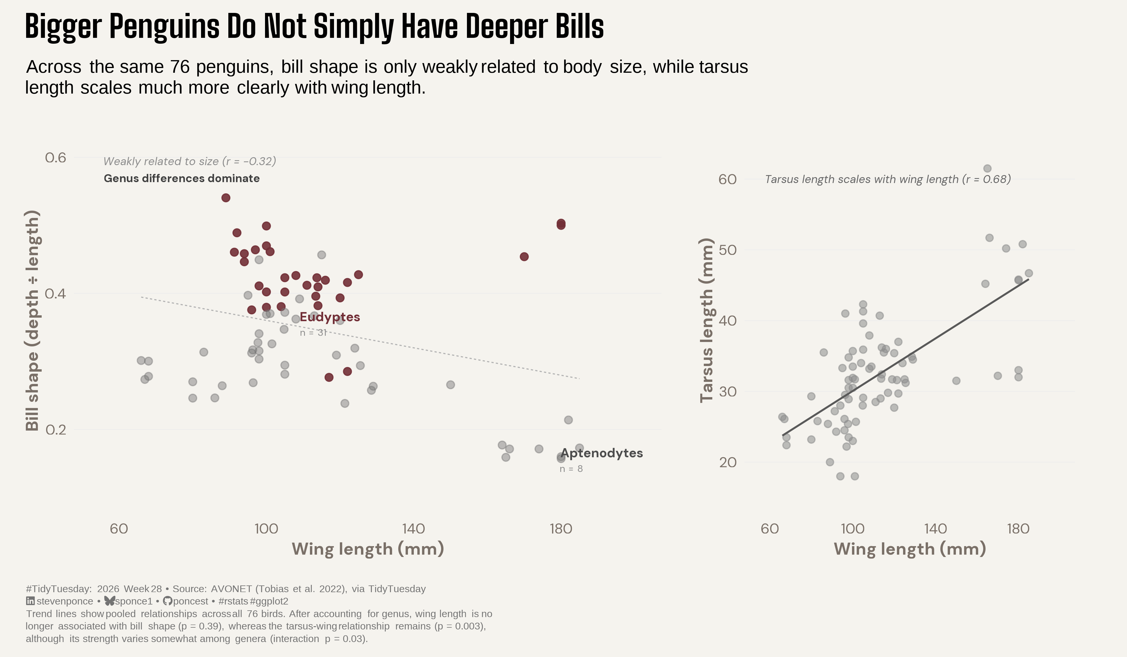
Across the same 76 penguins, bill shape is only weakly related to body size, while tarsus length scales much more clearly with wing length.

A two-panel scatterplot showing that penguin bill shape is only weakly related to wing length (r = -0.32), with a genus-adjusted regression model finding no significant within-genus relationship. A control panel confirms tarsus length scales clearly with wing length (r = 0.68), showing bill shape is the exception, not the rule. Built in R with ggplot2, patchwork, and ggtext.

Figure 1: Two-panel chart almost exactly on the diagonal reference line and an average calibration error of about 1 percentage point. Data from the fightr R package (UFC athlete profiles, UFCStats, Kaggle, Octagon API).

Steps to Create this Graphic

1. Load Packages & Setup

```{r}
#| label: load
#| warning: false
#| message: false      
#| results: "hide"     

## 1. LOAD PACKAGES & SETUP ----
suppressPackageStartupMessages({
if (!require("pacman")) install.packages("pacman")
pacman::p_load(
    tidyverse, ggtext, showtext, janitor, ggrepel,      
    scales, glue, skimr, patchwork
    )
})

### |- figure size ----          
camcorder::gg_record(
  dir    = here::here("temp_plots"),
    device = "png",
    width  = 12,
    height = 7,
    units  = "in",
    dpi    = 320
)

# Source utility functions
suppressMessages(source(here::here("R/utils/fonts.R")))
source(here::here("R/utils/social_icons.R"))
source(here::here("R/utils/image_utils.R"))
source(here::here("R/themes/base_theme.R"))
```

2. Read in the Data

```{r}
#| label: read
#| include: true
#| eval: true
#| warning: false

## 2. READ IN THE DATA ----
tt <- tidytuesdayR::tt_load(2026, week = 28)
many_penguins <- tt$many_penguins |> clean_names()
rm(tt)
```

3. Examine the Data

```{r}
#| label: examine
#| include: true
#| eval: true
#| results: 'hide'
#| warning: false

glimpse(many_penguins)
```

4. Tidy Data

```{r}
#| label: tidy
#| warning: false

penguins_shape <- many_penguins |>
  mutate(
    beak_shape_ratio = beak_depth / beak_length_culmen,
    is_highlight = genus == "Eudyptes"
  ) |>
  filter(
    !is.na(beak_shape_ratio),
    !is.na(wing_length),
    !is.na(tarsus_length)
  )

### |- genus cluster centers for direct labeling ----
genus_summary <- penguins_shape |>
  summarise(
    x_mean = mean(wing_length),
    y_mean = mean(beak_shape_ratio),
    n = n(),
    .by = genus
  ) |>
  arrange(desc(y_mean)) |>
  mutate(is_highlight = genus == "Eudyptes")

# Label only the two anchors
genus_labels <- genus_summary |>
  filter(genus %in% c("Eudyptes", "Aptenodytes")) |>
  mutate(
    label_x = case_when(
      genus == "Eudyptes" ~ 108,
      genus == "Aptenodytes" ~ x_mean + 4
    ),
    label_y = case_when(
      genus == "Eudyptes" ~ 0.355,
      genus == "Aptenodytes" ~ y_mean - 0.018
    )
  )

### |- correlation annotations
r_shape <- cor(penguins_shape$wing_length, penguins_shape$beak_shape_ratio) |> round(2)
r_tarsus <- cor(penguins_shape$wing_length, penguins_shape$tarsus_length) |> round(2)
n_total <- nrow(penguins_shape)
```

5. Visualization Parameters

```{r}
#| label: params
#| include: true
#| warning: false

### |- plot aesthetics ----
clrs <- get_theme_colors(
  palette = c("highlight" = "#722F37", "muted" = "gray70", "control" = "gray55")
)

### |- titles and caption ----
title_text <- str_glue("Bigger Penguins Do Not Simply Have Deeper Bills")

subtitle_text <- str_glue(
  "Across the same 76 penguins, bill shape is only weakly related to body ",
  "size, while tarsus length scales much more clearly with wing length."
) |>
  str_wrap(width = 95) |>
  str_replace_all("\n", "<br>")

caption_text <- str_glue(
  "{create_social_caption(tt_year = 2026, tt_week = 28, source_text = 'AVONET (Tobias et al. 2022), via TidyTuesday')}<br>",
  "{str_wrap(
    paste(
      'Trend lines show pooled relationships across all 76 birds. After accounting',
      'for genus, wing length is no longer associated with bill shape (p = 0.39),',
      'whereas the tarsus-wing relationship remains (p = 0.003), although its',
      'strength varies somewhat among genera (interaction p = 0.03).'
    ),
    width = 110
  ) |> str_replace_all('\n', '<br>')}"
)

### |- fonts ----
setup_fonts()
fonts <- get_font_families()

### |- plot theme ----
base_theme <- create_base_theme(clrs)

weekly_theme <- extend_weekly_theme(
  base_theme,
  theme(
    plot.title = element_text(
      face = "bold", size = rel(1.7), family = fonts$title_1
    ),
    plot.subtitle = element_markdown(
      size = rel(1.0), family = 'sans', lineheight = 1.15,
      margin = margin(t = 4, b = 12)
    ),
    plot.caption = element_markdown(
      size = rel(0.55), family = 'sans', color = "gray45",
      lineheight = 1.25, hjust = 0,
      margin = margin(t = 10)
    ),
    panel.grid.major.y = element_line(color = "gray93", linewidth = 0.25),
    panel.grid.major.x = element_blank(),
    panel.grid.minor = element_blank(),
    axis.ticks = element_blank(),
    legend.position = "none",
    plot.margin = margin(t = 10, r = 20, b = 10, l = 10)
  )
)

theme_set(weekly_theme)
```

6. Plot

```{r}
#| label: plot
#| warning: false

### |- plot ----

### |- panel A: bill shape ratio vs wing length ----
p_shape <- ggplot(penguins_shape, aes(x = wing_length, y = beak_shape_ratio)) +
  geom_point(
    aes(color = is_highlight, alpha = is_highlight),
    size = 2.4
  ) +
  geom_smooth(
    method = "lm", se = FALSE, color = "gray70",
    linewidth = 0.4, linetype = "22"
  ) +
  geom_richtext(
    data = genus_labels,
    aes(
      x = label_x, y = label_y,
      label = glue(
        "<span style='font-size:10pt;color:{ifelse(is_highlight, \"#722F37\", \"gray30\")}'>",
        "<b>{genus}</b></span><br>",
        "<span style='font-size:7.5pt;color:gray55'>n = {n}</span>"
      )
    ),
    hjust = 0, vjust = 0.5, lineheight = 1.0,
    family = fonts$text,
    fill = NA, label.color = NA,
    show.legend = FALSE
  ) +
  scale_color_manual(values = c("TRUE" = "#722F37", "FALSE" = "gray45")) +
  scale_alpha_manual(values = c("TRUE" = 0.9, "FALSE" = 0.45)) +
  scale_x_continuous(limits = c(55, 200), breaks = seq(60, 200, 40)) +
  scale_y_continuous(limits = c(0.1, 0.62), labels = label_number(accuracy = 0.1)) +
  labs(
    title = NULL,
    x = "Wing length (mm)",
    y = "Bill shape (depth \u00f7 length)"
  ) +
  annotate(
    "text",
    x = 56, y = 0.60,
    label = "Weakly related to size (r = -0.32)",
    hjust = 0, vjust = 1, size = 3, color = "gray55", fontface = "italic",
    family = fonts$text
  ) +
  annotate(
    "text",
    x = 56, y = 0.575,
    label = "Genus differences dominate",
    hjust = 0, vjust = 1, size = 3, color = "gray25", fontface = "bold",
    family = fonts$text
  )

### |- panel B: tarsus length vs wing length ----
p_control <- ggplot(penguins_shape, aes(x = wing_length, y = tarsus_length)) +
  geom_point(color = "gray55", alpha = 0.55, size = 2.2) +
  geom_smooth(
    method = "lm", se = FALSE, color = "gray35",
    linewidth = 0.7
  ) +
  scale_x_continuous(limits = c(55, 200), breaks = seq(60, 200, 40)) +
  scale_y_continuous(limits = c(15, 65)) +
  labs(
    title = NULL,
    x = "Wing length (mm)",
    y = "Tarsus length (mm)"
  ) +
  annotate(
    "text",
    x = 58, y = 60,
    label = glue("Tarsus length scales with wing length (r = {r_tarsus})"),
    hjust = 0, size = 3, color = "gray40", fontface = "italic",
    family = fonts$text, lineheight = 0.9
  )

### |- compose with patchwork  ----
combined_plot <- p_shape + p_control +
  plot_layout(widths = c(1.28, 0.72)) +
  plot_annotation(
    title = title_text,
    subtitle = subtitle_text,
    caption = caption_text,
    theme = weekly_theme
  )
```

7. Save

```{r}
#| label: save
#| warning: false

### |-  plot image ----  
save_plot_patchwork(
  plot = combined_plot, 
  type = "tidytuesday", 
  year = 2026, 
  week = 28, 
  width  = 12,
  height = 7
  )
```

8. Session Info

TipExpand for Session Info

R version 4.5.3 (2026-03-11 ucrt)
Platform: x86_64-w64-mingw32/x64
Running under: Windows 11 x64 (build 26100)

Matrix products: default
  LAPACK version 3.12.1

locale:
[1] LC_COLLATE=English_United States.utf8 
[2] LC_CTYPE=English_United States.utf8   
[3] LC_MONETARY=English_United States.utf8
[4] LC_NUMERIC=C                          
[5] LC_TIME=English_United States.utf8    

time zone: America/New_York
tzcode source: internal

attached base packages:
[1] stats     graphics  grDevices utils     datasets  methods   base     

other attached packages:
 [1] here_1.0.2      patchwork_1.3.2 skimr_2.2.2     glue_1.8.0     
 [5] scales_1.4.0    ggrepel_0.9.8   janitor_2.2.1   showtext_0.9-8 
 [9] showtextdb_3.0  sysfonts_0.8.9  ggtext_0.1.2    lubridate_1.9.5
[13] forcats_1.0.1   stringr_1.6.0   dplyr_1.2.1     purrr_1.2.2    
[17] readr_2.2.0     tidyr_1.3.2     tibble_3.3.1    ggplot2_4.0.3  
[21] tidyverse_2.0.0 pacman_0.5.1   

loaded via a namespace (and not attached):
 [1] tidyselect_1.2.1   farver_2.1.2       S7_0.2.1           fastmap_1.2.0     
 [5] gh_1.5.0           digest_0.6.39      timechange_0.4.0   lifecycle_1.0.5   
 [9] rsvg_2.7.0         magrittr_2.0.5     compiler_4.5.3     rlang_1.2.0       
[13] tools_4.5.3        yaml_2.3.12        knitr_1.51         labeling_0.4.3    
[17] htmlwidgets_1.6.4  bit_4.6.0          curl_7.0.0         xml2_1.5.2        
[21] camcorder_0.1.0    repr_1.1.7         RColorBrewer_1.1-3 tidytuesdayR_1.3.2
[25] withr_3.0.2        grid_4.5.3         gitcreds_0.1.2     cli_3.6.6         
[29] rmarkdown_2.31     crayon_1.5.3       generics_0.1.4     otel_0.2.0        
[33] rstudioapi_0.18.0  tzdb_0.5.0         commonmark_2.0.0   splines_4.5.3     
[37] parallel_4.5.3     ggplotify_0.1.3    base64enc_0.1-6    vctrs_0.7.3       
[41] yulab.utils_0.2.4  Matrix_1.7-4       jsonlite_2.0.0     litedown_0.9      
[45] gridGraphics_0.5-1 hms_1.1.4          bit64_4.6.0-1      systemfonts_1.3.2 
[49] magick_2.9.1       gifski_1.32.0-2    codetools_0.2-20   stringi_1.8.7     
[53] gtable_0.3.6       pillar_1.11.1      rappdirs_0.3.4     htmltools_0.5.9   
[57] R6_2.6.1           httr2_1.2.2        textshaping_1.0.5  rprojroot_2.1.1   
[61] lattice_0.22-9     vroom_1.7.1        evaluate_1.0.5     markdown_2.0      
[65] gridtext_0.1.6     snakecase_0.11.1   Rcpp_1.1.1         nlme_3.1-168      
[69] svglite_2.2.2      mgcv_1.9-4         xfun_0.57          fs_2.0.1          
[73] pkgconfig_2.0.3   

9. GitHub Repository

TipExpand for GitHub Repo

The complete code for this analysis is available in tt_2026_28.qmd.

For the full repository, click here.

10. References

TipExpand for References

1. Data Source:
   • TidyTuesday 2026 Week 28: Many Penguins

11. Custom Functions Documentation

Note📦 Custom Helper Functions

This analysis uses custom functions from my personal module library for efficiency and consistency across projects.

Functions Used:

• fonts.R: setup_fonts(), get_font_families() - Font management with showtext
• social_icons.R: create_social_caption() - Generates formatted social media captions
• image_utils.R: save_plot() - Consistent plot saving with naming conventions
• base_theme.R: create_base_theme(), extend_weekly_theme(), get_theme_colors() - Custom ggplot2 themes

Why custom functions?
These utilities standardize theming, fonts, and output across all my data visualizations. The core analysis (data tidying and visualization logic) uses only standard tidyverse packages.

Source Code:
View all custom functions → GitHub: R/utils