Out-of-body experiences are linked to ESP—not to unity

How much more common was each feature when an out-of-body experience was also reported?

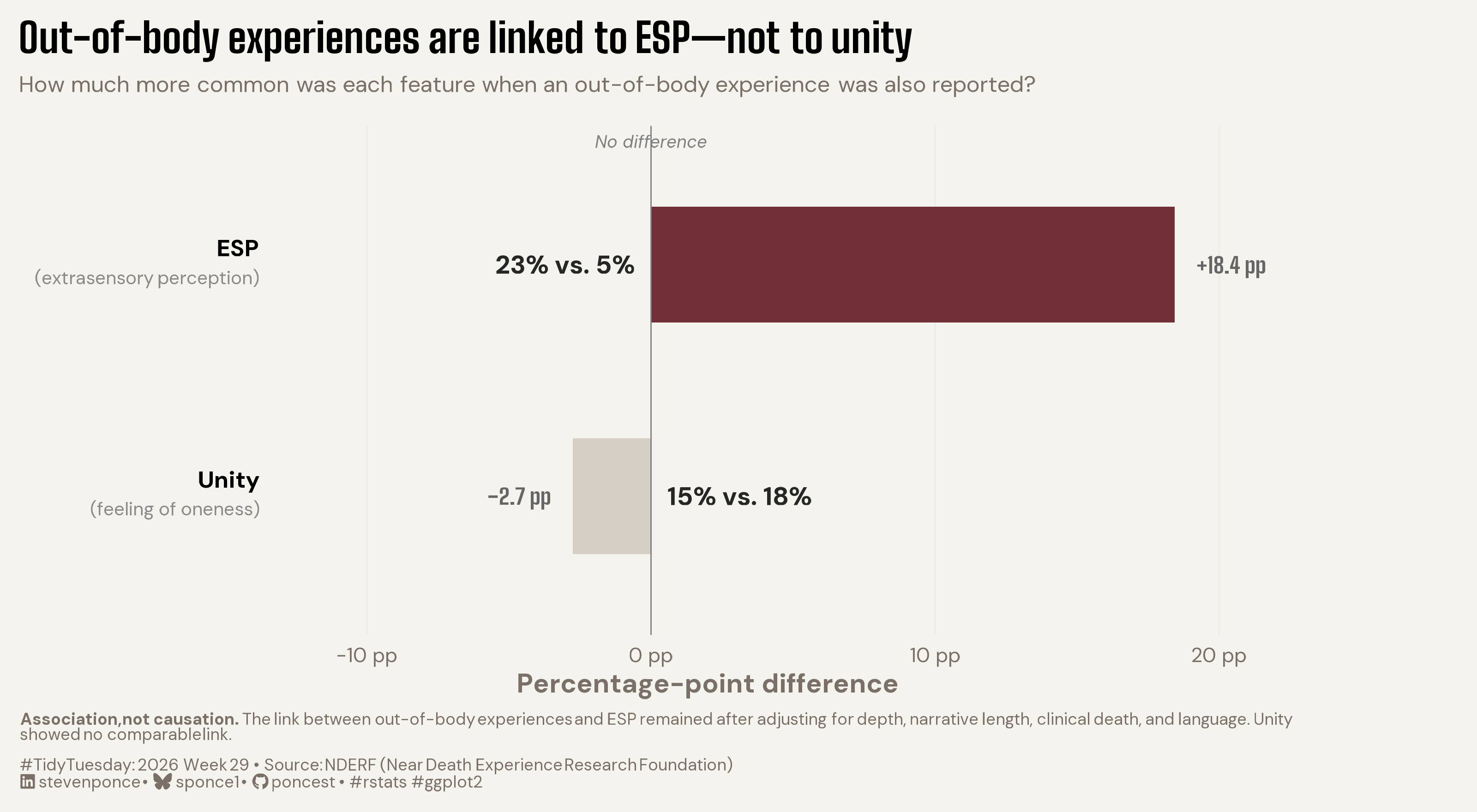
A percentage-point delta chart compares ESP and unity reporting rates between near-death accounts with and without a reported out-of-body experience. The ESP association held after adjusting for experience depth, narrative length, reported clinical death, and narrative language; the unity association did not. Built in R with ggplot2 and ggtext.

Figure 1: A delta bar chart titled “Out-of-body experiences are linked to ESP—not to unity.” Two horizontal bars show the percentage-point difference in reporting rates between near-death accounts with and without a reported out-of-body experience. The ESP bar extends 18.4 percentage points to the right, from 5% reporting ESP without an out-of-body experience to 23% with one. The Unity bar extends only 2.7 percentage points to the left, from 18% to 15%, shown in muted beige to signal no meaningful association. A caption notes the ESP link remained after adjusting for experience depth, narrative length, reported clinical death, and narrative language, while no comparable link was found for unity. Data from the NDERF near-death experience archive.

Steps to Create this Graphic

1. Load Packages & Setup

```{r}
#| label: load
#| warning: false
#| message: false      
#| results: "hide"     

## 1. LOAD PACKAGES & SETUP ----
suppressPackageStartupMessages({
if (!require("pacman")) install.packages("pacman")
pacman::p_load(
    tidyverse, ggtext, showtext, janitor, ggrepel,      
    scales, glue, skimr
    )
})

### |- figure size ----          
camcorder::gg_record(
  dir    = here::here("temp_plots"),
    device = "png",
    width  = 10,
    height = 5.5,
    units  = "in",
    dpi    = 320
)

# Source utility functions
suppressMessages(source(here::here("R/utils/fonts.R")))
source(here::here("R/utils/social_icons.R"))
source(here::here("R/utils/image_utils.R"))
source(here::here("R/themes/base_theme.R"))
```

2. Read in the Data

```{r}
#| label: read
#| include: true
#| eval: true
#| warning: false

## 2. READ IN THE DATA ----
tt <- tidytuesdayR::tt_load(2026, week = 29)
nde_experiences <- tt$nde_experiences |> clean_names()
rm(tt)
```

3. Examine the Data

```{r}
#| label: examine
#| include: true
#| eval: true
#| results: 'hide'
#| warning: false

glimpse(nde_experiences)
```

4. Tidy Data

```{r}
#| label: tidy
#| warning: false

### |- analytic sample ----
nde_clean <- nde_experiences |>
    filter(!is.na(greyson_score))

### |- Wilson CI helper ----
wilson_ci <- function(x, n, conf = 0.95) {
    z <- qnorm(1 - (1 - conf) / 2)
    p <- x / n
    denom <- 1 + z^2 / n
    center <- (p + z^2 / (2 * n)) / denom
    half <- z * sqrt(p * (1 - p) / n + z^2 / (4 * n^2)) / denom
    tibble(estimate = p, conf.low = center - half, conf.high = center + half)
}

### |- raw comparison table (OBE present/absent x ESP/Unity) ----
raw_summary <- nde_clean |>
    mutate(obe_group = if_else(ai_obe, "OBE reported", "No OBE reported")) |>
    summarise(
        n = n(),
        esp_x = sum(ai_esp),
        unity_x = sum(ai_unity),
        .by = obe_group
    ) |>
    mutate(
        esp = map2(esp_x, n, wilson_ci),
        unity = map2(unity_x, n, wilson_ci)
    ) |>
    select(obe_group, n, esp, unity) |>
    pivot_longer(c(esp, unity), names_to = "feature", values_to = "ci") |>
    unnest(ci) |>
    mutate(
        feature = case_match(feature, "esp" ~ "ESP", "unity" ~ "Unity"),
        obe_group = factor(obe_group, levels = c("No OBE reported", "OBE reported"))
    )

### |- delta table ----
delta_summary <- raw_summary |>
    select(feature, obe_group, estimate) |>
    pivot_wider(names_from = obe_group, values_from = estimate) |>
    mutate(
        delta = `OBE reported` - `No OBE reported`,
        delta_label = glue("{if_else(delta >= 0, '+', '\u2212')}{abs(round(delta * 100, 1))} pp"),
        raw_label = glue(
            "{percent(`OBE reported`, accuracy = 1)} vs. {percent(`No OBE reported`, accuracy = 1)}"
        ),
        bar_color = if_else(feature == "ESP", "#722F37", "#C2B8AC"),  
        bar_alpha = if_else(feature == "ESP", 1, 0.6),          
        gloss_label = case_match(
            feature,
            "ESP"   ~ "**ESP**<br><span style='font-size:9pt;color:#8A8A8A'>(extrasensory perception)</span>",
            "Unity" ~ "**Unity**<br><span style='font-size:9pt;color:#8A8A8A'>(feeling of oneness)</span>"
        ),
        feature = factor(feature, levels = c("Unity", "ESP")),
        y_pos = as.integer(feature)   
    )
```

5. Visualization Parameters

```{r}
#| label: params
#| include: true
#| warning: false

### |- plot aesthetics ----
colors <- get_theme_colors(
    palette = c("highlight" = "#722F37", "muted" = "#C2B8AC")
)

### |- titles and caption ----
title_text <- str_wrap(
    "Out-of-body experiences are linked to ESP—not to unity",
    width = 55
) |> str_replace_all("\n", "<br>")

subtitle_text <- str_glue(
    "How much more common was each feature when an out-of-body experience was also reported?"
)

footnote_text <- str_wrap(
    "**Association, not causation.** The link between out-of-body experiences and ESP remained after adjusting for depth, narrative length, clinical death, and language. Unity showed no comparable link.",
    width = 175
) |> str_replace_all("\n", "<br>")

caption_text <- create_social_caption(
    tt_year = 2026,
    tt_week = 29,
    source_text = "NDERF (Near Death Experience Research Foundation)"
)

### |- fonts ----
setup_fonts()
fonts <- get_font_families()

### |- plot theme ----
base_theme <- create_base_theme(colors)

weekly_theme <- extend_weekly_theme(
    base_theme,
    theme(
        plot.title = element_markdown(face = "bold", family = fonts$title_1, size = 20, lineheight = 1.15),
        plot.subtitle = element_markdown(family = fonts$text, size = 11, margin = margin(b = 14), color = colors$subtitle),
        plot.caption = element_markdown(family = fonts$text, size = 8, hjust = 0, color = colors$caption),
        plot.margin = margin(t = 10, r = 40, b = 10, l = 10),
        panel.grid.major.y = element_blank(),
        panel.grid.major.x = element_line(color = "gray92", linewidth = 0.3),
        panel.grid.minor = element_blank(),
        axis.ticks = element_blank(),
        axis.text.y = element_blank(),  
        axis.text.x = element_text(size = 10)
    )
)

theme_set(weekly_theme)
```

6. Plot

```{r}
#| label: plot
#| warning: false

### |- plot ----
p <- delta_summary |>
    ggplot(aes(x = delta, y = feature)) +
    geom_col(aes(fill = bar_color, alpha = bar_alpha), width = 0.5) +
    geom_vline(xintercept = 0, color = "gray50", linewidth = 0.3) +
    annotate(
        "text", x = 0, y = Inf, label = "No difference",
        size = 3, family = fonts$text, color = "gray50", fontface = "italic",
        hjust = 0.5, vjust = 1.8
    ) +
    scale_fill_identity() +
    scale_alpha_identity() +
    geom_richtext(
        aes(x = -0.135, y = y_pos, label = gloss_label),
        hjust = 1, vjust = 0.5,
        family = fonts$text, size = 4,
        fill = NA, label.color = NA,
        inherit.aes = FALSE, data = delta_summary
    ) +
    geom_text(
        aes(
            label = delta_label,
            x = delta + if_else(delta >= 0, 0.008, -0.008),
            hjust = if_else(delta >= 0, 0, 1)
        ),
        size = 3.8, fontface = "bold", family = fonts$title_1, color = "gray40"
    ) +
    geom_text(
        aes(label = raw_label, x = 0, hjust = if_else(delta >= 0, 1, 0)),
        nudge_x = if_else(delta_summary$delta >= 0, -0.006, 0.006),
        size = 4.4, fontface = "bold", family = fonts$text, color = "gray15"
    ) +
    scale_x_continuous(
        limits = c(-0.2, 0.24),
        labels = label_number(suffix = " pp", scale = 100),
        breaks = c(-0.10, 0, 0.10, 0.20)
    ) +
    coord_cartesian(clip = "off") +
    labs(
        title = title_text,
        subtitle = subtitle_text,
        caption = glue("{footnote_text}<br><br>{caption_text}"),
        x = "Percentage-point difference", y = NULL
    )
```

7. Save

```{r}
#| label: save
#| warning: false

### |-  plot image ----  
save_plot(
  plot = p, 
  type = "tidytuesday", 
  year = 2026, 
  week = 29, 
  width  = 10,
  height = 5.5
  )
```

8. Session Info

TipExpand for Session Info

R version 4.6.1 (2026-06-24)
Platform: aarch64-apple-darwin23
Running under: macOS Tahoe 26.5.2

Matrix products: default
BLAS:   /Library/Frameworks/R.framework/Versions/4.6/Resources/lib/libRblas.0.dylib 
LAPACK: /Library/Frameworks/R.framework/Versions/4.6/Resources/lib/libRlapack.dylib;  LAPACK version 3.12.1

locale:
[1] en_US.UTF-8/en_US.UTF-8/en_US.UTF-8/C/en_US.UTF-8/en_US.UTF-8

time zone: America/New_York
tzcode source: internal

attached base packages:
[1] stats     graphics  grDevices utils     datasets  methods   base     

other attached packages:
 [1] here_1.0.2      skimr_2.2.2     glue_1.8.1      scales_1.4.0   
 [5] ggrepel_0.9.8   janitor_2.2.1   showtext_0.9-8  showtextdb_3.0 
 [9] sysfonts_0.8.9  ggtext_0.1.2    lubridate_1.9.5 forcats_1.0.1  
[13] stringr_1.6.0   dplyr_1.2.1     purrr_1.2.2     readr_2.2.0    
[17] tidyr_1.3.2     tibble_3.3.1    ggplot2_4.0.3   tidyverse_2.0.0
[21] pacman_0.5.1   

loaded via a namespace (and not attached):
 [1] generics_0.1.4     xml2_1.6.0         stringi_1.8.7      hms_1.1.4         
 [5] digest_0.6.39      magrittr_2.0.5     evaluate_1.0.5     grid_4.6.1        
 [9] timechange_0.4.0   RColorBrewer_1.1-3 fastmap_1.2.0      rprojroot_2.1.1   
[13] jsonlite_2.0.0     codetools_0.2-20   textshaping_1.0.5  cli_3.6.6         
[17] rlang_1.3.0        litedown_0.10      commonmark_2.0.0   base64enc_0.1-6   
[21] repr_1.1.7         withr_3.0.3        yaml_2.3.12        otel_0.2.0        
[25] tools_4.6.1        tzdb_0.5.0         vctrs_0.7.3        R6_2.6.1          
[29] magick_2.9.1       lifecycle_1.0.5    snakecase_0.11.1   htmlwidgets_1.6.4 
[33] ragg_1.5.2         pkgconfig_2.0.3    pillar_1.11.1      gtable_0.3.6      
[37] Rcpp_1.1.2         systemfonts_1.3.2  xfun_0.60          tidyselect_1.2.1  
[41] rstudioapi_0.19.0  knitr_1.51         farver_2.1.2       htmltools_0.5.9   
[45] rmarkdown_2.31     compiler_4.6.1     S7_0.2.2           markdown_2.0      
[49] gridtext_0.1.6    

9. GitHub Repository

TipExpand for GitHub Repo

The complete code for this analysis is available in tt_2026_29.qmd.

For the full repository, click here.

10. References

TipExpand for References

1. Data Source:
   • TidyTuesday 2026 Week 29: Near-Death Experiences (NDERF)

11. Custom Functions Documentation

Note📦 Custom Helper Functions

This analysis uses custom functions from my personal module library for efficiency and consistency across projects.

Functions Used:

• fonts.R: setup_fonts(), get_font_families() - Font management with showtext
• social_icons.R: create_social_caption() - Generates formatted social media captions
• image_utils.R: save_plot() - Consistent plot saving with naming conventions
• base_theme.R: create_base_theme(), extend_weekly_theme(), get_theme_colors() - Custom ggplot2 themes

Why custom functions?
These utilities standardize theming, fonts, and output across all my data visualizations. The core analysis (data tidying and visualization logic) uses only standard tidyverse packages.

Source Code:
View all custom functions → GitHub: R/utils