• Steven Ponce
  • About
  • Data Visualizations
  • Projects
  • Resume
  • Email

On this page

  • Steps to Create this Graphic
    • 1. Load Packages & Setup
    • 2. Read in the Data
    • 3. Examine the Data
    • 4. Tidy Data
    • 5. Visualization Parameters
    • 6. Plot
    • 7. Save
    • 8. Session Info
    • 9. GitHub Repository
    • 10. References
    • 11. Custom Functions Documentation

Different climates, less distinct local weather

  • Show All Code
  • Hide All Code

  • View Source

How geography and local seasonal baselines changed the apparent weather patterns in Australian ecotourism observations

TidyTuesday
Data Visualization
R Programming
2026
A TidyTuesday analysis showing how large raw temperature differences across four species shrink substantially after accounting for each weather station’s local seasonal normal. Uses a leave-one-out day-of-year baseline and deduplicated species × station × date units to correct for geography and repeated logging. Built in R with ggplot2, ggridges, and patchwork.
Author

Steven Ponce

Published

July 24, 2026

Figure 1: Paired ridgeline chart comparing observed temperatures with temperature departures from each weather station’s seasonal normal for orchids, manta rays, Gouldian finches, and glowworms. The species occupy markedly different raw temperature ranges, but their local temperature anomalies overlap much more. Glowworm is shown as five individual points because only five station-days were available.

Steps to Create this Graphic

1. Load Packages & Setup

Show code
```{r}
#| label: load
#| warning: false
#| message: false      
#| results: "hide"     

## 1. LOAD PACKAGES & SETUP ----
suppressPackageStartupMessages({
if (!require("pacman")) install.packages("pacman")
pacman::p_load(
    tidyverse, ggtext, showtext, janitor, ggrepel,      
    scales, glue, skimr, patchwork, ggridges
    )
})

### |- figure size ----          
camcorder::gg_record(
  dir    = here::here("temp_plots"),
    device = "png",
    width  = 11,
    height = 6.5,
    units  = "in",
    dpi    = 320
)

# Source utility functions
suppressMessages(source(here::here("R/utils/fonts.R")))
source(here::here("R/utils/social_icons.R"))
source(here::here("R/utils/image_utils.R"))
source(here::here("R/themes/base_theme.R"))
```

2. Read in the Data

Show code
```{r}
#| label: read
#| include: true
#| eval: true
#| warning: false

## 2. READ IN THE DATA ----
tt <- tidytuesdayR::tt_load(2026, week = 30)
occurrences <- tt$occurrences |> clean_names()
weather     <- tt$weather     |> clean_names()
rm(tt)
```

3. Examine the Data

Show code
```{r}
#| label: examine
#| include: true
#| eval: true
#| results: 'hide'
#| warning: false

glimpse(occurrences)
glimpse(weather)
```

4. Tidy Data

Show code
```{r}
#| label: tidy
#| warning: false

## |- join, explicit suffixes ----
occ_weather <- occurrences |>
  left_join(weather, by = c("date", "ws_id"), suffix = c("_occ", "_wx"))

### |- leave-one-out day-of-year baseline ----
weather_loo <- weather |>
  left_join(
    weather |>
      summarise(
        baseline_sum = sum(temp, na.rm = TRUE),
        baseline_n = sum(!is.na(temp)),
        .by = c(ws_id, dayofyear)
      ),
    by = c("ws_id", "dayofyear")
  ) |>
  mutate(
    temp_baseline_loo = case_when(
      !is.na(temp) & baseline_n > 1 ~ (baseline_sum - temp) / (baseline_n - 1),
      TRUE ~ NA_real_
    ),
    temp_anomaly_loo = temp - temp_baseline_loo
  )

occ_weather_loo <- occ_weather |>
  left_join(
    weather_loo |> select(ws_id, date, temp_anomaly_loo),
    by = c("ws_id", "date")
  )

### |- dedup to species x station x date ----
species_station_days <- occ_weather_loo |>
  filter(!is.na(temp), !is.na(temp_anomaly_loo)) |>
  summarise(
    temp = first(temp),
    temp_anomaly = first(temp_anomaly_loo),
    .by = c(organism_name, ws_id, date)
  )

### |- species order + sample-size labels ----
species_order <- species_station_days |>
  summarise(median_temp = median(temp), n = n(), .by = organism_name) |>
  arrange(median_temp) |>
  mutate(label = glue::glue("{organism_name} (n={n})"))

### |- attach ordered species label ----
species_station_days <- species_station_days |>
  left_join(species_order |> select(organism_name, label), by = "organism_name") |>
  mutate(label = factor(label, levels = species_order$label))

### |- split ridgeline species vs. sparse-observation species ----
glowworm_label <- species_order$label[species_order$organism_name == "Glowworm"]

ridge_data <- species_station_days |> filter(organism_name != "Glowworm")
sparse_data <- species_station_days |> filter(organism_name == "Glowworm")
```

5. Visualization Parameters

Show code
```{r}
#| label: params
#| include: true
#| warning: false

### |- plot aesthetics ----
clrs <- get_theme_colors(
    palette = list(
        col_glowworm = "gray55",
        col_orchid   = "#4A7A96",
        col_manta    = "#C98A3C",
        col_gouldian = "#722F37"
    )
)

## literal hex values here instead of extracting from clrs.
species_palette <- c("gray55", "#4A7A96", "#C98A3C", "#722F37")[
    seq_along(levels(species_station_days$label))
]
names(species_palette) <- levels(species_station_days$label)

### |- fonts ----
setup_fonts()
fonts <- get_font_families()

### |- titles and caption ----
title_text    <- "Different climates, less distinct local weather"

subtitle_text <- paste0(
    "Observed temperatures span nearly 20\u00b0C across species \u2014<br>",
    "comparing each station-day with its own seasonal normal removes much of the apparent separation."
)

### |- footnote + social caption ----
footnote_line1 <- str_wrap(
    "**Left: **temperature on observed station-days. **Right: **departure from each station's day-of-year average. One observation was retained per species \u00d7 station \u00d7 date. Glowworm is shown as points because only five station-days were available.",
    width = 100) |> str_replace_all("\n", "<br>")

footnote_line2 <- "Limited station coverage prevents species-level inference."

footnote_text <- paste0(footnote_line1, "<br>", footnote_line2)

social_caption <- create_social_caption(
    tt_year = 2026,
    tt_week = 30,
    source_text = "ecotourism R package (occurrences, weather, and tourism data)"
)

caption_text <- paste0(footnote_text, "<br><br>", social_caption)

### |- plot theme ----
base_theme <- create_base_theme(clrs)

weekly_theme <- extend_weekly_theme(
  base_theme,
  theme(
    plot.title = element_markdown(face = "bold", family = fonts$title_1, size = 24, lineheight = 1.15),
    plot.subtitle = element_markdown(family = fonts$text, size = 11, margin = margin(b = 14), lineheight = 1.1, color = "#4A4340"),
    plot.caption = element_markdown(family = fonts$caption, size = 6, hjust = 0, color = "#7A7068", lineheight = 1.4),
    plot.margin = margin(t = 10, r = 40, b = 10, l = 10),
    panel.grid.major.y = element_blank(),
    panel.grid.major.x = element_line(color = "gray92", linewidth = 0.3),
    panel.grid.minor = element_blank(),
    axis.ticks = element_blank(),
    axis.text.x = element_text(size = 10)
  )
)

theme_set(weekly_theme)
```

6. Plot

Show code
```{r}
#| label: plot
#| warning: false

### |- panel A: climate where observed ----
p_raw <- ggplot(species_station_days, aes(y = label)) +
  annotate("segment",
    x = -Inf, xend = Inf, y = glowworm_label, yend = glowworm_label,
    color = "gray88", linewidth = 0.4
  ) +
  geom_density_ridges(
    data = ridge_data, aes(x = temp, fill = label),
    color = "white", alpha = 0.9, scale = 0.95
  ) +
  geom_point(
    data = sparse_data, aes(x = temp, color = label),
    size = 2.4, alpha = 0.9
  ) +
  scale_fill_manual(values = species_palette, guide = "none") +
  scale_color_manual(values = species_palette, guide = "none") +
  scale_x_continuous(labels = label_number(suffix = "\u00b0C")) +
  labs(title = "Climate where observed", x = NULL, y = NULL) +
  theme(
    plot.title.position = "panel",
    plot.title = element_markdown(
      family = fonts$text, size = 12, color = "gray30",
      hjust = 0.5, face = "plain"
    ),
    axis.text.y = element_text(family = fonts$text, face = "bold", size = 10, color = "gray20")
  )

### |- panel B: relative to local seasonal normal ----
p_anomaly <- ggplot(species_station_days, aes(y = label)) +
  annotate("segment",
    x = -Inf, xend = Inf, y = glowworm_label, yend = glowworm_label,
    color = "gray88", linewidth = 0.4
  ) +
  geom_vline(xintercept = 0, color = "gray50", linewidth = 0.4, linetype = "dashed", alpha = 0.55) +
  geom_density_ridges(
    data = ridge_data, aes(x = temp_anomaly, fill = label),
    color = "white", alpha = 0.9, scale = 0.95
  ) +
  geom_point(
    data = sparse_data, aes(x = temp_anomaly, color = label),
    size = 2.4, alpha = 0.9
  ) +
  scale_fill_manual(values = species_palette, guide = "none") +
  scale_color_manual(values = species_palette, guide = "none") +
  scale_x_continuous(labels = label_number(suffix = "\u00b0C", style_positive = "plus")) +
  labs(title = "Relative to local seasonal normal", x = NULL, y = NULL) +
  theme(
    plot.title.position = "panel",
    plot.title = element_markdown(
      family = fonts$text, size = 12, color = "gray30",
      hjust = 0.5, face = "plain"
    ),
    axis.text.y = element_blank()
  )

### |- combine ----
p <- (p_raw | p_anomaly) +
  plot_annotation(
    title = title_text,
    subtitle = subtitle_text,
    caption = caption_text
  )
```

7. Save

Show code
```{r}
#| label: save
#| warning: false

camcorder::gg_stop_recording()

save_plot_patchwork(
  plot = p,
  type = "tidytuesday",
  year = 2026,
  week = 30,
  width  = 11,
  height = 6.5
)
```

8. Session Info

TipExpand for Session Info
R version 4.6.1 (2026-06-24)
Platform: aarch64-apple-darwin23
Running under: macOS Tahoe 26.5.2

Matrix products: default
BLAS:   /Library/Frameworks/R.framework/Versions/4.6/Resources/lib/libRblas.0.dylib 
LAPACK: /Library/Frameworks/R.framework/Versions/4.6/Resources/lib/libRlapack.dylib;  LAPACK version 3.12.1

locale:
[1] en_US.UTF-8/en_US.UTF-8/en_US.UTF-8/C/en_US.UTF-8/en_US.UTF-8

time zone: America/New_York
tzcode source: internal

attached base packages:
[1] stats     graphics  grDevices utils     datasets  methods   base     

other attached packages:
 [1] here_1.0.2      ggridges_0.5.7  patchwork_1.3.2 skimr_2.2.2    
 [5] glue_1.8.1      scales_1.4.0    ggrepel_0.9.8   janitor_2.2.1  
 [9] showtext_0.9-8  showtextdb_3.0  sysfonts_0.8.9  ggtext_0.1.2   
[13] lubridate_1.9.5 forcats_1.0.1   stringr_1.6.0   dplyr_1.2.1    
[17] purrr_1.2.2     readr_2.2.0     tidyr_1.3.2     tibble_3.3.1   
[21] ggplot2_4.0.3   tidyverse_2.0.0 pacman_0.5.1   

loaded via a namespace (and not attached):
 [1] gtable_0.3.6       httr2_1.3.0        xfun_0.60          htmlwidgets_1.6.4 
 [5] gh_1.6.1           tzdb_0.5.0         vctrs_0.7.3        tools_4.6.1       
 [9] generics_0.1.4     parallel_4.6.1     curl_7.1.0         gifski_1.32.0-2   
[13] pkgconfig_2.0.3    RColorBrewer_1.1-3 S7_0.2.2           lifecycle_1.0.5   
[17] compiler_4.6.1     farver_2.1.2       textshaping_1.0.5  repr_1.1.7        
[21] codetools_0.2-20   snakecase_0.11.1   litedown_0.10      htmltools_0.5.9   
[25] yaml_2.3.12        crayon_1.5.3       pillar_1.11.1      camcorder_0.1.0   
[29] magick_2.9.1       commonmark_2.0.0   tidyselect_1.2.1   digest_0.6.39     
[33] stringi_1.8.7      labeling_0.4.3     rsvg_2.7.0         rprojroot_2.1.1   
[37] fastmap_1.2.0      grid_4.6.1         cli_3.6.6          magrittr_2.0.5    
[41] base64enc_0.1-6    withr_3.0.3        bit64_4.8.2        timechange_0.4.0  
[45] tidytuesdayR_1.3.2 rmarkdown_2.31     gitcreds_0.1.2     bit_4.6.0         
[49] otel_0.2.0         ragg_1.5.2         hms_1.1.4          evaluate_1.0.5    
[53] knitr_1.51         markdown_2.0       rlang_1.3.0        gridtext_0.1.6    
[57] Rcpp_1.1.2         xml2_1.6.0         vroom_1.7.1        svglite_2.2.2     
[61] rstudioapi_0.19.0  jsonlite_2.0.0     R6_2.6.1           systemfonts_1.3.2 

9. GitHub Repository

TipExpand for GitHub Repo

The complete code for this analysis is available in tt_2026_30.qmd.

For the full repository, click here.

10. References

TipExpand for References
  1. Data Source:
    • TidyTuesday 2026 Week 30: Ecotourism

11. Custom Functions Documentation

Note📦 Custom Helper Functions

This analysis uses custom functions from my personal module library for efficiency and consistency across projects.

Functions Used:

  • fonts.R: setup_fonts(), get_font_families() - Font management with showtext
  • social_icons.R: create_social_caption() - Generates formatted social media captions
  • image_utils.R: save_plot() - Consistent plot saving with naming conventions
  • base_theme.R: create_base_theme(), extend_weekly_theme(), get_theme_colors() - Custom ggplot2 themes

Why custom functions?
These utilities standardize theming, fonts, and output across all my data visualizations. The core analysis (data tidying and visualization logic) uses only standard tidyverse packages.

Source Code:
View all custom functions → GitHub: R/utils

Back to top

Citation

BibTeX citation:
@online{ponce2026,
  author = {Ponce, Steven},
  title = {Different Climates, Less Distinct Local Weather},
  date = {2026-07-24},
  url = {https://stevenponce.netlify.app/data_visualizations/TidyTuesday/2026/tt_2026_30.html},
  langid = {en}
}
For attribution, please cite this work as:
Ponce, Steven. 2026. “Different Climates, Less Distinct Local Weather.” July 24. https://stevenponce.netlify.app/data_visualizations/TidyTuesday/2026/tt_2026_30.html.
Source Code
---
title: "Different climates, less distinct local weather"
subtitle: "How geography and local seasonal baselines changed the apparent weather patterns in Australian ecotourism observations"
description: "A TidyTuesday analysis showing how large raw temperature differences across four species shrink substantially after accounting for each weather station's local seasonal normal. Uses a leave-one-out day-of-year baseline and deduplicated species × station × date units to correct for geography and repeated logging. Built in R with ggplot2, ggridges, and patchwork."
date: "2026-07-24"
author:
  - name: "Steven Ponce"
    url: "https://stevenponce.netlify.app"
citation:
  url: "https://stevenponce.netlify.app/data_visualizations/TidyTuesday/2026/tt_2026_30.html"
categories: ["TidyTuesday", "Data Visualization", "R Programming", "2026"]
tags: [
  "TidyTuesday",
  "Ridgeline Chart",
  "ggridges",
  "patchwork",
  "ecology",
  "ecotourism",
  "Australia",
  "weather",
  "seasonal-anomaly",
  "geography",
  "distribution-comparison",
  "data-storytelling",
  "R",
  "2026"
]
image: "thumbnails/tt_2026_30.png"
format:
  html:
    toc: true
    toc-depth: 5
    code-link: true
    code-fold: true
    code-tools: true
    code-summary: "Show code"
    self-contained: true
    theme: 
      light: [flatly, assets/styling/custom_styles.scss]
      dark: [darkly, assets/styling/custom_styles_dark.scss]
editor_options: 
  chunk_output_type: inline
execute: 
  freeze: true
  cache: true
  error: false
  message: false
  warning: false
  eval: true
---
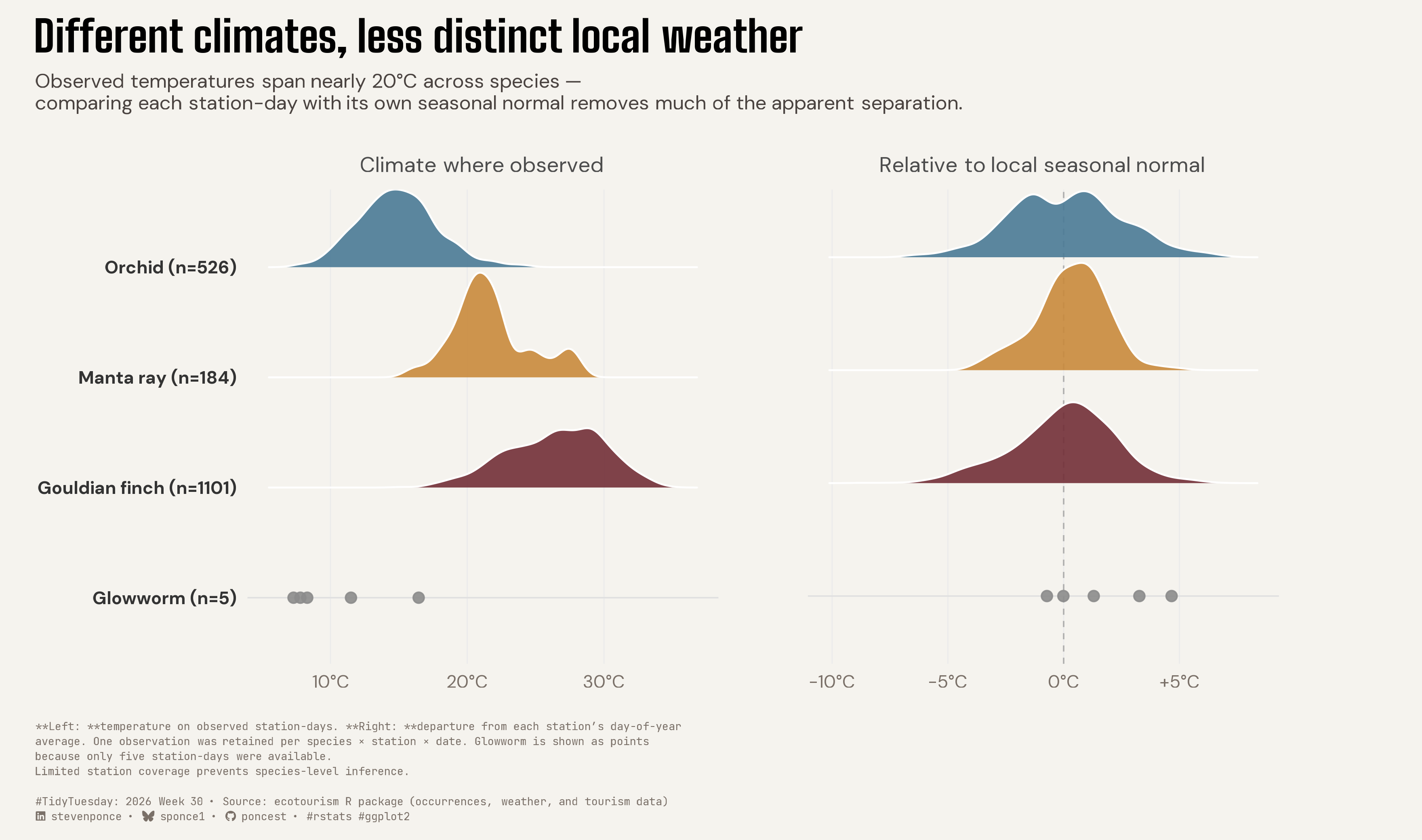
![Paired ridgeline chart comparing observed temperatures with temperature departures from each weather station's seasonal normal for orchids, manta rays, Gouldian finches, and glowworms. The species occupy markedly different raw temperature ranges, but their local temperature anomalies overlap much more. Glowworm is shown as five individual points because only five station-days were available.](tt_2026_30.png){#fig-1}

### [**Steps to Create this Graphic**]{.mark}

#### [1. Load Packages & Setup]{.smallcaps}

```{r}
#| label: load
#| warning: false
#| message: false      
#| results: "hide"     

## 1. LOAD PACKAGES & SETUP ----
suppressPackageStartupMessages({
if (!require("pacman")) install.packages("pacman")
pacman::p_load(
    tidyverse, ggtext, showtext, janitor, ggrepel,      
    scales, glue, skimr, patchwork, ggridges
    )
})

### |- figure size ----          
camcorder::gg_record(
  dir    = here::here("temp_plots"),
    device = "png",
    width  = 11,
    height = 6.5,
    units  = "in",
    dpi    = 320
)

# Source utility functions
suppressMessages(source(here::here("R/utils/fonts.R")))
source(here::here("R/utils/social_icons.R"))
source(here::here("R/utils/image_utils.R"))
source(here::here("R/themes/base_theme.R"))
```

#### [2. Read in the Data]{.smallcaps}

```{r}
#| label: read
#| include: true
#| eval: true
#| warning: false

## 2. READ IN THE DATA ----
tt <- tidytuesdayR::tt_load(2026, week = 30)
occurrences <- tt$occurrences |> clean_names()
weather     <- tt$weather     |> clean_names()
rm(tt)
```

#### [3. Examine the Data]{.smallcaps}

```{r}
#| label: examine
#| include: true
#| eval: true
#| results: 'hide'
#| warning: false

glimpse(occurrences)
glimpse(weather)
```

#### [4. Tidy Data]{.smallcaps}

```{r}
#| label: tidy
#| warning: false

## |- join, explicit suffixes ----
occ_weather <- occurrences |>
  left_join(weather, by = c("date", "ws_id"), suffix = c("_occ", "_wx"))

### |- leave-one-out day-of-year baseline ----
weather_loo <- weather |>
  left_join(
    weather |>
      summarise(
        baseline_sum = sum(temp, na.rm = TRUE),
        baseline_n = sum(!is.na(temp)),
        .by = c(ws_id, dayofyear)
      ),
    by = c("ws_id", "dayofyear")
  ) |>
  mutate(
    temp_baseline_loo = case_when(
      !is.na(temp) & baseline_n > 1 ~ (baseline_sum - temp) / (baseline_n - 1),
      TRUE ~ NA_real_
    ),
    temp_anomaly_loo = temp - temp_baseline_loo
  )

occ_weather_loo <- occ_weather |>
  left_join(
    weather_loo |> select(ws_id, date, temp_anomaly_loo),
    by = c("ws_id", "date")
  )

### |- dedup to species x station x date ----
species_station_days <- occ_weather_loo |>
  filter(!is.na(temp), !is.na(temp_anomaly_loo)) |>
  summarise(
    temp = first(temp),
    temp_anomaly = first(temp_anomaly_loo),
    .by = c(organism_name, ws_id, date)
  )

### |- species order + sample-size labels ----
species_order <- species_station_days |>
  summarise(median_temp = median(temp), n = n(), .by = organism_name) |>
  arrange(median_temp) |>
  mutate(label = glue::glue("{organism_name} (n={n})"))

### |- attach ordered species label ----
species_station_days <- species_station_days |>
  left_join(species_order |> select(organism_name, label), by = "organism_name") |>
  mutate(label = factor(label, levels = species_order$label))

### |- split ridgeline species vs. sparse-observation species ----
glowworm_label <- species_order$label[species_order$organism_name == "Glowworm"]

ridge_data <- species_station_days |> filter(organism_name != "Glowworm")
sparse_data <- species_station_days |> filter(organism_name == "Glowworm")

```

#### [5. Visualization Parameters]{.smallcaps}

```{r}
#| label: params
#| include: true
#| warning: false

### |- plot aesthetics ----
clrs <- get_theme_colors(
    palette = list(
        col_glowworm = "gray55",
        col_orchid   = "#4A7A96",
        col_manta    = "#C98A3C",
        col_gouldian = "#722F37"
    )
)

## literal hex values here instead of extracting from clrs.
species_palette <- c("gray55", "#4A7A96", "#C98A3C", "#722F37")[
    seq_along(levels(species_station_days$label))
]
names(species_palette) <- levels(species_station_days$label)

### |- fonts ----
setup_fonts()
fonts <- get_font_families()

### |- titles and caption ----
title_text    <- "Different climates, less distinct local weather"

subtitle_text <- paste0(
    "Observed temperatures span nearly 20\u00b0C across species \u2014<br>",
    "comparing each station-day with its own seasonal normal removes much of the apparent separation."
)

### |- footnote + social caption ----
footnote_line1 <- str_wrap(
    "**Left: **temperature on observed station-days. **Right: **departure from each station's day-of-year average. One observation was retained per species \u00d7 station \u00d7 date. Glowworm is shown as points because only five station-days were available.",
    width = 100) |> str_replace_all("\n", "<br>")

footnote_line2 <- "Limited station coverage prevents species-level inference."

footnote_text <- paste0(footnote_line1, "<br>", footnote_line2)

social_caption <- create_social_caption(
    tt_year = 2026,
    tt_week = 30,
    source_text = "ecotourism R package (occurrences, weather, and tourism data)"
)

caption_text <- paste0(footnote_text, "<br><br>", social_caption)

### |- plot theme ----
base_theme <- create_base_theme(clrs)

weekly_theme <- extend_weekly_theme(
  base_theme,
  theme(
    plot.title = element_markdown(face = "bold", family = fonts$title_1, size = 24, lineheight = 1.15),
    plot.subtitle = element_markdown(family = fonts$text, size = 11, margin = margin(b = 14), lineheight = 1.1, color = "#4A4340"),
    plot.caption = element_markdown(family = fonts$caption, size = 6, hjust = 0, color = "#7A7068", lineheight = 1.4),
    plot.margin = margin(t = 10, r = 40, b = 10, l = 10),
    panel.grid.major.y = element_blank(),
    panel.grid.major.x = element_line(color = "gray92", linewidth = 0.3),
    panel.grid.minor = element_blank(),
    axis.ticks = element_blank(),
    axis.text.x = element_text(size = 10)
  )
)

theme_set(weekly_theme)
```

#### [6. Plot]{.smallcaps}

```{r}
#| label: plot
#| warning: false

### |- panel A: climate where observed ----
p_raw <- ggplot(species_station_days, aes(y = label)) +
  annotate("segment",
    x = -Inf, xend = Inf, y = glowworm_label, yend = glowworm_label,
    color = "gray88", linewidth = 0.4
  ) +
  geom_density_ridges(
    data = ridge_data, aes(x = temp, fill = label),
    color = "white", alpha = 0.9, scale = 0.95
  ) +
  geom_point(
    data = sparse_data, aes(x = temp, color = label),
    size = 2.4, alpha = 0.9
  ) +
  scale_fill_manual(values = species_palette, guide = "none") +
  scale_color_manual(values = species_palette, guide = "none") +
  scale_x_continuous(labels = label_number(suffix = "\u00b0C")) +
  labs(title = "Climate where observed", x = NULL, y = NULL) +
  theme(
    plot.title.position = "panel",
    plot.title = element_markdown(
      family = fonts$text, size = 12, color = "gray30",
      hjust = 0.5, face = "plain"
    ),
    axis.text.y = element_text(family = fonts$text, face = "bold", size = 10, color = "gray20")
  )

### |- panel B: relative to local seasonal normal ----
p_anomaly <- ggplot(species_station_days, aes(y = label)) +
  annotate("segment",
    x = -Inf, xend = Inf, y = glowworm_label, yend = glowworm_label,
    color = "gray88", linewidth = 0.4
  ) +
  geom_vline(xintercept = 0, color = "gray50", linewidth = 0.4, linetype = "dashed", alpha = 0.55) +
  geom_density_ridges(
    data = ridge_data, aes(x = temp_anomaly, fill = label),
    color = "white", alpha = 0.9, scale = 0.95
  ) +
  geom_point(
    data = sparse_data, aes(x = temp_anomaly, color = label),
    size = 2.4, alpha = 0.9
  ) +
  scale_fill_manual(values = species_palette, guide = "none") +
  scale_color_manual(values = species_palette, guide = "none") +
  scale_x_continuous(labels = label_number(suffix = "\u00b0C", style_positive = "plus")) +
  labs(title = "Relative to local seasonal normal", x = NULL, y = NULL) +
  theme(
    plot.title.position = "panel",
    plot.title = element_markdown(
      family = fonts$text, size = 12, color = "gray30",
      hjust = 0.5, face = "plain"
    ),
    axis.text.y = element_blank()
  )

### |- combine ----
p <- (p_raw | p_anomaly) +
  plot_annotation(
    title = title_text,
    subtitle = subtitle_text,
    caption = caption_text
  )
```

#### [7. Save]{.smallcaps}

```{r}
#| label: save
#| warning: false

camcorder::gg_stop_recording()

save_plot_patchwork(
  plot = p,
  type = "tidytuesday",
  year = 2026,
  week = 30,
  width  = 11,
  height = 6.5
)
```

#### [8. Session Info]{.smallcaps}

::: {.callout-tip collapse="true"}
##### Expand for Session Info

```{r, echo = FALSE}
#| eval: true
#| warning: false

sessionInfo()
```
:::

#### [9. GitHub Repository]{.smallcaps}

::: {.callout-tip collapse="true"}
##### Expand for GitHub Repo

The complete code for this analysis is available in [`tt_2026_30.qmd`](https://github.com/poncest/personal-website/blob/master/data_visualizations/TidyTuesday/2026/tt_2026_30.qmd).

For the full repository, [click here](https://github.com/poncest/personal-website/).
:::

#### [10. References]{.smallcaps}

::: {.callout-tip collapse="true"}
##### Expand for References
1.  **Data Source:**
    -   TidyTuesday 2026 Week 30: [Ecotourism](https://github.com/rfordatascience/tidytuesday/blob/main/data/2026/2026-07-28/readme.md)

:::


#### [11. Custom Functions Documentation]{.smallcaps}

::: {.callout-note collapse="true"}
##### 📦 Custom Helper Functions

This analysis uses custom functions from my personal module library for efficiency and consistency across projects.

**Functions Used:**

-   **`fonts.R`**: `setup_fonts()`, `get_font_families()` - Font management with showtext
-   **`social_icons.R`**: `create_social_caption()` - Generates formatted social media captions
-   **`image_utils.R`**: `save_plot()` - Consistent plot saving with naming conventions
-   **`base_theme.R`**: `create_base_theme()`, `extend_weekly_theme()`, `get_theme_colors()` - Custom ggplot2 themes

**Why custom functions?**\
These utilities standardize theming, fonts, and output across all my data visualizations. The core analysis (data tidying and visualization logic) uses only standard tidyverse packages.

**Source Code:**\
View all custom functions → [GitHub: R/utils](https://github.com/poncest/personal-website/tree/master/R)
:::

© 2024 Steven Ponce

Source Issues