• Steven Ponce
  • About
  • Data Visualizations
  • Projects
  • Resume
  • Email

On this page

  • Steps to Create this Graphic
    • 1. Load Packages & Setup
    • 2. Read in the Data
    • 3. Examine the Data
    • 4. Tidy Data
    • 5. Visualization Parameters
    • 6. Plot
  • 7. Save
    • 8. Session Info
    • 9. GitHub Repository
    • 10. References
    • 11. Custom Functions Documentation

Different climates, less distinct local weather

  • Show All Code
  • Hide All Code

  • View Source

How geography and local seasonal baselines changed the apparent weather patterns in Australian ecotourism observations

TidyTuesday
Data Visualization
R Programming
2026
A TidyTuesday analysis showing how large raw temperature differences across four species shrink substantially after accounting for each weather station’s local seasonal normal. Uses a leave-one-out day-of-year baseline and deduplicated species × station × date units to correct for geography and repeated logging. Built in R with ggplot2, ggridges, and patchwork.
Author

Steven Ponce

Published

August 1, 2026

Figure 1: Two-panel bar chart, “One Producer, Two Calendars.” Each bar shows a month’s trade value as a percent deviation from that importer’s own average, 2016–2024. Top panel: South Africa’s Basotho wool imports peak in October–November (about +150%) and trough April–July (down to -93%). Bottom panel: China’s imports peak in April (+133%) and trough August–October (down to -88%, based on only 4–6 annual observations). The same wool follows opposite seasonal calendars depending on destination. Data are partner-reported imports from Lesotho via UN Comtrade, not export or shearing records.

Steps to Create this Graphic

1. Load Packages & Setup

Show code
```{r}
#| label: load
#| warning: false
#| message: false      
#| results: "hide"     

## 1. LOAD PACKAGES & SETUP ----
suppressPackageStartupMessages({
if (!require("pacman")) install.packages("pacman")
pacman::p_load(
    tidyverse, ggtext, showtext, janitor, ggrepel,      
    scales, glue, skimr, ggview
    )
})

# Source utility functions
suppressMessages(source(here::here("R/utils/fonts.R")))
source(here::here("R/utils/social_icons.R"))
source(here::here("R/utils/image_utils.R"))
source(here::here("R/themes/base_theme.R"))
```

2. Read in the Data

Show code
```{r}
#| label: read
#| include: true
#| eval: true
#| warning: false

## 2. READ IN THE DATA ----
tt <- tidytuesdayR::tt_load(2026, week = 31)
basotho_wool <- tt$basotho_wool |> clean_names()
rm(tt)
```

3. Examine the Data

Show code
```{r}
#| label: examine
#| include: true
#| eval: true
#| results: 'hide'
#| warning: false

glimpse(basotho_wool)
skim_without_charts(basotho_wool)
```

4. Tidy Data

Show code
```{r}
#| label: tidy
#| warning: false

## |- Restrict to the two reporters with sufficient monthly density ----
wool_only <- basotho_wool |> filter(cmd_code == 5101)

wool_compare <- wool_only |>
  filter(
    reporter_desc %in% c("South Africa", "China"),
    ref_year >= 2016
  ) |>
  summarise(
    total_value = sum(primary_value, na.rm = TRUE),
    .by = c(reporter_desc, ref_month)
  )

## |- Seasonal deviation, signed: % above/below the reporter's OWN average month ----
seasonal_profile <- wool_compare |>
  mutate(
    reporter_mean = mean(total_value),
    pct_deviation = (total_value / reporter_mean - 1) * 100,
    .by = reporter_desc
  ) |>
  mutate(
    month_abb = factor(month.abb[ref_month], levels = month.abb),
    reporter_desc = factor(reporter_desc, levels = c("South Africa", "China"))
  )

## |- n ----
china_thin <- wool_only |>
  filter(reporter_desc == "China") |>
  count(ref_month) |>
  filter(n <= 6) |>
  arrange(ref_month)

china_caveat_label <- str_glue(
  "{first(month.abb[china_thin$ref_month])}\u2013",
  "{last(month.abb[china_thin$ref_month])} based on only ",
  "{min(china_thin$n)}\u2013{max(china_thin$n)} annual observations"
)
```

5. Visualization Parameters

Show code
```{r}
#| label: params
#| include: true
#| warning: false

## |-  plot aesthetics ----
clrs <- get_theme_colors(
  palette = c(
    "South Africa" = "#722F37",
    "China"        = "#A8B4BC"
  )
)

col_south_africa <- "#722F37"
col_china <- "#A8B4BC"

### |-  titles and caption ----
title_text <- str_glue("One Producer, Two Calendars")

subtitle_text <- str_glue(
  "Basotho wool imported by South Africa peaks in **Oct–Nov**,<br>",
  "while imports reported by **China** follow a sharply different ",
  "seasonal rhythm."
)
caption_explainer <- str_wrap(
  paste(
    "Both panels use the shared 2016\u20132024 reporting window.",
    "Oct\u2013Nov corresponds to spring in Lesotho (Southern Hemisphere).",
    "The data show when importing countries report the wool, not when it",
    "was shorn, sold, or shipped."
  ),
  width = 110
) |>
  str_replace_all("\n", "<br>")

caption_text <- str_glue(
  "{caption_explainer}<br>",
  create_social_caption(
    tt_year = 2026,
    tt_week = 31,
    source_text = "UN Comtrade via comtradr · partner-reported imports from Lesotho"
  )
)

### |-  fonts ----
setup_fonts()
fonts <- get_font_families()

### |-  plot theme ----
base_theme <- create_base_theme(clrs)

weekly_theme <- extend_weekly_theme(
  base_theme,
  theme(
    plot.title = element_text(
      face = "bold", size = rel(1.6), family = fonts$title_1,
      margin = margin(b = 8), fonts$title_1, color = clrs$title
    ),
    plot.subtitle = element_markdown(
      size = rel(0.8), family = fonts$subtitle, lineheight = 1.15,
      margin = margin(b = 16), color = clrs$subtitle
    ),
    plot.caption = element_markdown(
      size = rel(0.5), family = fonts$caption, color = alpha(clrs$caption, 0.8) 
    ),
    strip.text = element_text(
      face = "bold", size = rel(1.05), family = fonts$title_2, hjust = 0
    ),
    panel.grid.major.y = element_line(color = "gray90", linewidth = 0.3),
    panel.grid.major.x = element_blank(),
    panel.grid.minor = element_blank(),
    axis.ticks = element_blank(),
    axis.text.y = element_text(size = rel(0.7)),
    legend.position = "none"
  )
)

theme_set(weekly_theme)
```

6. Plot

Show code
```{r}
#| label: plot
#| warning: false

### |- plot----
p <- ggplot(seasonal_profile, aes(x = month_abb, y = pct_deviation, fill = reporter_desc)) +
  geom_col(width = 0.72) +
  geom_hline(yintercept = 0, color = "gray40", linewidth = 0.4) +
  geom_text(
    data = tibble(
      reporter_desc = factor("South Africa", levels = levels(seasonal_profile$reporter_desc)),
      x_pos = 10.5,
      pct_deviation = 185,
      label = "Peak"
    ),
    aes(x = x_pos, y = pct_deviation, label = label),
    inherit.aes = FALSE,
    family = fonts$text, size = 3.1, color = col_south_africa,
    fontface = "italic", hjust = 0.5
  ) +
  geom_text(
    data = tibble(
      reporter_desc = factor("China", levels = levels(seasonal_profile$reporter_desc)),
      x_pos = 9,
      pct_deviation = -118,
      label = china_caveat_label
    ),
    aes(x = x_pos, y = pct_deviation, label = label),
    inherit.aes = FALSE,
    family = fonts$text, size = 2.8, color = "gray30", fontface = "bold.italic"
  ) +
  facet_wrap(~reporter_desc, ncol = 1) +
  scale_fill_manual(
    values = c("South Africa" = col_south_africa, "China" = col_china)
  ) +
  scale_y_continuous(
    labels = \(x) paste0(ifelse(x > 0, "+", ""), x, "%"),
    breaks = seq(-100, 200, 50),
    expand = expansion(mult = c(0.08, 0.12))
  ) +
  labs(
    title = title_text,
    subtitle = subtitle_text,
    caption = caption_text,
    x = NULL,
    y = "Monthly deviation from each importer's average"
  ) +
  canvas(width = 8, height = 8.7, units = "in", dpi = 300)
```

7. Save

Show code
```{r}
#| label: save
#| warning: false

### |- save ----
main_path  <- here::here("data_visualizations", "TidyTuesday", "2026", "tt_2026_31.png")
thumb_path <- here::here("data_visualizations", "TidyTuesday", "2026", "thumbnails", "tt_2026_31.png")

# Full-size version, for the QMD figure
save_ggplot(
  plot = p,
  file = main_path,
  width = 8,
  height = 8.7,
  units = "in",
  dpi = 320,
  create.dir = TRUE
)

# Reduced-size thumbnail, for the YAML `image:` field
fs::dir_create(dirname(thumb_path))
magick::image_read(main_path) |>
  magick::image_resize("400") |>
  magick::image_write(thumb_path)
```

8. Session Info

TipExpand for Session Info
R version 4.6.1 (2026-06-24)
Platform: aarch64-apple-darwin23
Running under: macOS Tahoe 26.5.2

Matrix products: default
BLAS:   /Library/Frameworks/R.framework/Versions/4.6/Resources/lib/libRblas.0.dylib 
LAPACK: /Library/Frameworks/R.framework/Versions/4.6/Resources/lib/libRlapack.dylib;  LAPACK version 3.12.1

locale:
[1] en_US.UTF-8/en_US.UTF-8/en_US.UTF-8/C/en_US.UTF-8/en_US.UTF-8

time zone: America/New_York
tzcode source: internal

attached base packages:
[1] stats     graphics  grDevices utils     datasets  methods   base     

other attached packages:
 [1] here_1.0.2      ggview_0.2.2    skimr_2.2.2     glue_1.8.1     
 [5] scales_1.4.0    ggrepel_0.9.8   janitor_2.2.1   showtext_0.9-8 
 [9] showtextdb_3.0  sysfonts_0.8.9  ggtext_0.1.2    lubridate_1.9.5
[13] forcats_1.0.1   stringr_1.6.0   dplyr_1.2.1     purrr_1.2.2    
[17] readr_2.2.0     tidyr_1.3.2     tibble_3.3.1    ggplot2_4.0.3  
[21] tidyverse_2.0.0 pacman_0.5.1   

loaded via a namespace (and not attached):
 [1] gtable_0.3.6       xfun_0.60          httr2_1.3.0        htmlwidgets_1.6.4 
 [5] gh_1.6.1           tzdb_0.5.0         vctrs_0.7.3        tools_4.6.1       
 [9] generics_0.1.4     parallel_4.6.1     curl_7.1.0         pkgconfig_2.0.3   
[13] RColorBrewer_1.1-3 S7_0.2.2           lifecycle_1.0.5    compiler_4.6.1    
[17] farver_2.1.2       textshaping_1.0.5  repr_1.1.7         codetools_0.2-20  
[21] snakecase_0.11.1   litedown_0.10      htmltools_0.5.9    yaml_2.3.12       
[25] crayon_1.5.3       pillar_1.11.1      commonmark_2.0.0   tidyselect_1.2.1  
[29] digest_0.6.39      stringi_1.8.7      rprojroot_2.1.1    fastmap_1.2.0     
[33] grid_4.6.1         cli_3.6.6          magrittr_2.0.5     base64enc_0.1-6   
[37] withr_3.0.3        bit64_4.8.2        timechange_0.4.0   rmarkdown_2.31    
[41] tidytuesdayR_1.3.2 gitcreds_0.1.2     bit_4.6.0          otel_0.2.0        
[45] ragg_1.5.2         hms_1.1.4          evaluate_1.0.5     knitr_1.51        
[49] markdown_2.0       rlang_1.3.0        gridtext_0.1.6     Rcpp_1.1.2        
[53] xml2_1.6.0         rstudioapi_0.19.0  vroom_1.7.1        jsonlite_2.0.0    
[57] R6_2.6.1           systemfonts_1.3.2 

9. GitHub Repository

TipExpand for GitHub Repo

The complete code for this analysis is available in tt_2026_31.qmd.

For the full repository, click here.

10. References

TipExpand for References
  1. Data Source:
    • TidyTuesday 2026 Week 31: Ecotourism

11. Custom Functions Documentation

Note📦 Custom Helper Functions

This analysis uses custom functions from my personal module library for efficiency and consistency across projects.

Functions Used:

  • fonts.R: setup_fonts(), get_font_families() - Font management with showtext
  • social_icons.R: create_social_caption() - Generates formatted social media captions
  • image_utils.R: save_plot() - Consistent plot saving with naming conventions
  • base_theme.R: create_base_theme(), extend_weekly_theme(), get_theme_colors() - Custom ggplot2 themes

Why custom functions?
These utilities standardize theming, fonts, and output across all my data visualizations. The core analysis (data tidying and visualization logic) uses only standard tidyverse packages.

Source Code:
View all custom functions → GitHub: R/utils

Back to top

Citation

BibTeX citation:
@online{ponce2026,
  author = {Ponce, Steven},
  title = {Different Climates, Less Distinct Local Weather},
  date = {2026-08-01},
  url = {https://stevenponce.netlify.app/data_visualizations/TidyTuesday/2026/tt_2026_31.html},
  langid = {en}
}
For attribution, please cite this work as:
Ponce, Steven. 2026. “Different Climates, Less Distinct Local Weather.” August 1. https://stevenponce.netlify.app/data_visualizations/TidyTuesday/2026/tt_2026_31.html.
Source Code
---
title: "Different climates, less distinct local weather"
subtitle: "How geography and local seasonal baselines changed the apparent weather patterns in Australian ecotourism observations"
description: "A TidyTuesday analysis showing how large raw temperature differences across four species shrink substantially after accounting for each weather station's local seasonal normal. Uses a leave-one-out day-of-year baseline and deduplicated species × station × date units to correct for geography and repeated logging. Built in R with ggplot2, ggridges, and patchwork."
date: "2026-08-01"
author:
  - name: "Steven Ponce"
    url: "https://stevenponce.netlify.app"
citation:
  url: "https://stevenponce.netlify.app/data_visualizations/TidyTuesday/2026/tt_2026_31.html"
categories: ["TidyTuesday", "Data Visualization", "R Programming", "2026"]
tags: [
  "TidyTuesday",
  "Ridgeline Chart",
  "ggridges",
  "patchwork",
  "ecology",
  "ecotourism",
  "Australia",
  "weather",
  "seasonal-anomaly",
  "geography",
  "distribution-comparison",
  "data-storytelling",
  "R",
  "2026"
]
image: "thumbnails/tt_2026_31.png"
format:
  html:
    toc: true
    toc-depth: 5
    code-link: true
    code-fold: true
    code-tools: true
    code-summary: "Show code"
    self-contained: true
    theme: 
      light: [flatly, assets/styling/custom_styles.scss]
      dark: [darkly, assets/styling/custom_styles_dark.scss]
editor_options: 
  chunk_output_type: inline
execute: 
  freeze: true
  cache: true
  error: false
  message: false
  warning: false
  eval: true
---
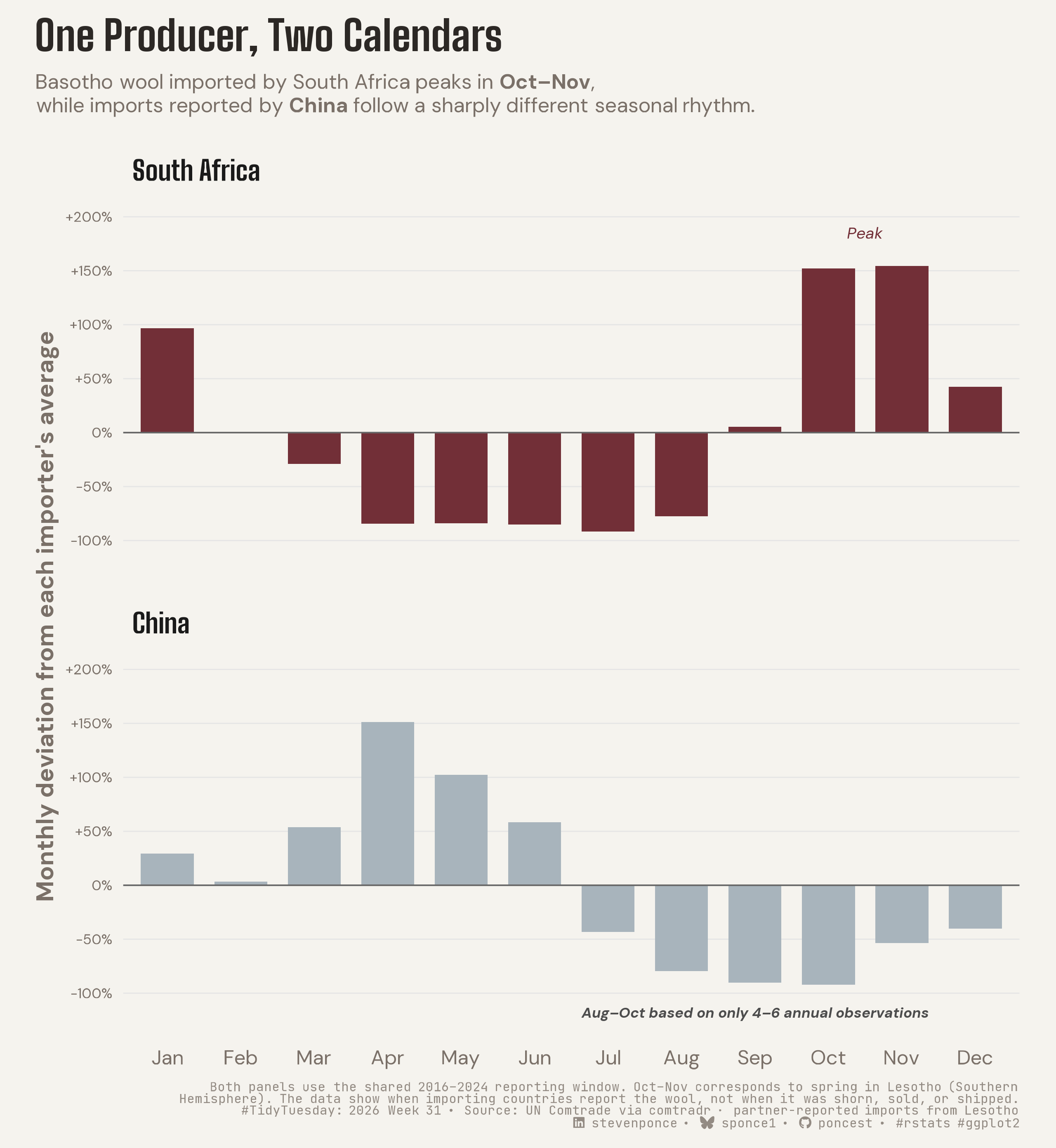
![Two-panel bar chart, "One Producer, Two Calendars." Each bar shows a month's trade value as a percent deviation from that importer's own average, 2016–2024. Top panel: South Africa's Basotho wool imports peak in October–November (about +150%) and trough April–July (down to -93%). Bottom panel: China's imports peak in April (+133%) and trough August–October (down to -88%, based on only 4–6 annual observations). The same wool follows opposite seasonal calendars depending on destination. Data are partner-reported imports from Lesotho via UN Comtrade, not export or shearing records.](tt_2026_31.png){#fig-1}

### [**Steps to Create this Graphic**]{.mark}

#### [1. Load Packages & Setup]{.smallcaps}

```{r}
#| label: load
#| warning: false
#| message: false      
#| results: "hide"     

## 1. LOAD PACKAGES & SETUP ----
suppressPackageStartupMessages({
if (!require("pacman")) install.packages("pacman")
pacman::p_load(
    tidyverse, ggtext, showtext, janitor, ggrepel,      
    scales, glue, skimr, ggview
    )
})

# Source utility functions
suppressMessages(source(here::here("R/utils/fonts.R")))
source(here::here("R/utils/social_icons.R"))
source(here::here("R/utils/image_utils.R"))
source(here::here("R/themes/base_theme.R"))
```

#### [2. Read in the Data]{.smallcaps}

```{r}
#| label: read
#| include: true
#| eval: true
#| warning: false

## 2. READ IN THE DATA ----
tt <- tidytuesdayR::tt_load(2026, week = 31)
basotho_wool <- tt$basotho_wool |> clean_names()
rm(tt)
```

#### [3. Examine the Data]{.smallcaps}

```{r}
#| label: examine
#| include: true
#| eval: true
#| results: 'hide'
#| warning: false

glimpse(basotho_wool)
skim_without_charts(basotho_wool)
```

#### [4. Tidy Data]{.smallcaps}

```{r}
#| label: tidy
#| warning: false

## |- Restrict to the two reporters with sufficient monthly density ----
wool_only <- basotho_wool |> filter(cmd_code == 5101)

wool_compare <- wool_only |>
  filter(
    reporter_desc %in% c("South Africa", "China"),
    ref_year >= 2016
  ) |>
  summarise(
    total_value = sum(primary_value, na.rm = TRUE),
    .by = c(reporter_desc, ref_month)
  )

## |- Seasonal deviation, signed: % above/below the reporter's OWN average month ----
seasonal_profile <- wool_compare |>
  mutate(
    reporter_mean = mean(total_value),
    pct_deviation = (total_value / reporter_mean - 1) * 100,
    .by = reporter_desc
  ) |>
  mutate(
    month_abb = factor(month.abb[ref_month], levels = month.abb),
    reporter_desc = factor(reporter_desc, levels = c("South Africa", "China"))
  )

## |- n ----
china_thin <- wool_only |>
  filter(reporter_desc == "China") |>
  count(ref_month) |>
  filter(n <= 6) |>
  arrange(ref_month)

china_caveat_label <- str_glue(
  "{first(month.abb[china_thin$ref_month])}\u2013",
  "{last(month.abb[china_thin$ref_month])} based on only ",
  "{min(china_thin$n)}\u2013{max(china_thin$n)} annual observations"
)
```

#### [5. Visualization Parameters]{.smallcaps}

```{r}
#| label: params
#| include: true
#| warning: false

## |-  plot aesthetics ----
clrs <- get_theme_colors(
  palette = c(
    "South Africa" = "#722F37",
    "China"        = "#A8B4BC"
  )
)

col_south_africa <- "#722F37"
col_china <- "#A8B4BC"

### |-  titles and caption ----
title_text <- str_glue("One Producer, Two Calendars")

subtitle_text <- str_glue(
  "Basotho wool imported by South Africa peaks in **Oct–Nov**,<br>",
  "while imports reported by **China** follow a sharply different ",
  "seasonal rhythm."
)
caption_explainer <- str_wrap(
  paste(
    "Both panels use the shared 2016\u20132024 reporting window.",
    "Oct\u2013Nov corresponds to spring in Lesotho (Southern Hemisphere).",
    "The data show when importing countries report the wool, not when it",
    "was shorn, sold, or shipped."
  ),
  width = 110
) |>
  str_replace_all("\n", "<br>")

caption_text <- str_glue(
  "{caption_explainer}<br>",
  create_social_caption(
    tt_year = 2026,
    tt_week = 31,
    source_text = "UN Comtrade via comtradr · partner-reported imports from Lesotho"
  )
)

### |-  fonts ----
setup_fonts()
fonts <- get_font_families()

### |-  plot theme ----
base_theme <- create_base_theme(clrs)

weekly_theme <- extend_weekly_theme(
  base_theme,
  theme(
    plot.title = element_text(
      face = "bold", size = rel(1.6), family = fonts$title_1,
      margin = margin(b = 8), fonts$title_1, color = clrs$title
    ),
    plot.subtitle = element_markdown(
      size = rel(0.8), family = fonts$subtitle, lineheight = 1.15,
      margin = margin(b = 16), color = clrs$subtitle
    ),
    plot.caption = element_markdown(
      size = rel(0.5), family = fonts$caption, color = alpha(clrs$caption, 0.8) 
    ),
    strip.text = element_text(
      face = "bold", size = rel(1.05), family = fonts$title_2, hjust = 0
    ),
    panel.grid.major.y = element_line(color = "gray90", linewidth = 0.3),
    panel.grid.major.x = element_blank(),
    panel.grid.minor = element_blank(),
    axis.ticks = element_blank(),
    axis.text.y = element_text(size = rel(0.7)),
    legend.position = "none"
  )
)

theme_set(weekly_theme)
```

#### [6. Plot]{.smallcaps}

```{r}
#| label: plot
#| warning: false

### |- plot----
p <- ggplot(seasonal_profile, aes(x = month_abb, y = pct_deviation, fill = reporter_desc)) +
  geom_col(width = 0.72) +
  geom_hline(yintercept = 0, color = "gray40", linewidth = 0.4) +
  geom_text(
    data = tibble(
      reporter_desc = factor("South Africa", levels = levels(seasonal_profile$reporter_desc)),
      x_pos = 10.5,
      pct_deviation = 185,
      label = "Peak"
    ),
    aes(x = x_pos, y = pct_deviation, label = label),
    inherit.aes = FALSE,
    family = fonts$text, size = 3.1, color = col_south_africa,
    fontface = "italic", hjust = 0.5
  ) +
  geom_text(
    data = tibble(
      reporter_desc = factor("China", levels = levels(seasonal_profile$reporter_desc)),
      x_pos = 9,
      pct_deviation = -118,
      label = china_caveat_label
    ),
    aes(x = x_pos, y = pct_deviation, label = label),
    inherit.aes = FALSE,
    family = fonts$text, size = 2.8, color = "gray30", fontface = "bold.italic"
  ) +
  facet_wrap(~reporter_desc, ncol = 1) +
  scale_fill_manual(
    values = c("South Africa" = col_south_africa, "China" = col_china)
  ) +
  scale_y_continuous(
    labels = \(x) paste0(ifelse(x > 0, "+", ""), x, "%"),
    breaks = seq(-100, 200, 50),
    expand = expansion(mult = c(0.08, 0.12))
  ) +
  labs(
    title = title_text,
    subtitle = subtitle_text,
    caption = caption_text,
    x = NULL,
    y = "Monthly deviation from each importer's average"
  ) +
  canvas(width = 8, height = 8.7, units = "in", dpi = 300)
```

### [7. Save]{.smallcaps}

```{r}
#| label: save
#| warning: false

### |- save ----
main_path  <- here::here("data_visualizations", "TidyTuesday", "2026", "tt_2026_31.png")
thumb_path <- here::here("data_visualizations", "TidyTuesday", "2026", "thumbnails", "tt_2026_31.png")

# Full-size version, for the QMD figure
save_ggplot(
  plot = p,
  file = main_path,
  width = 8,
  height = 8.7,
  units = "in",
  dpi = 320,
  create.dir = TRUE
)

# Reduced-size thumbnail, for the YAML `image:` field
fs::dir_create(dirname(thumb_path))
magick::image_read(main_path) |>
  magick::image_resize("400") |>
  magick::image_write(thumb_path)
```


#### [8. Session Info]{.smallcaps}

::: {.callout-tip collapse="true"}
##### Expand for Session Info

```{r, echo = FALSE}
#| eval: true
#| warning: false

sessionInfo()
```
:::

#### [9. GitHub Repository]{.smallcaps}

::: {.callout-tip collapse="true"}
##### Expand for GitHub Repo

The complete code for this analysis is available in [`tt_2026_31.qmd`](https://github.com/poncest/personal-website/blob/master/data_visualizations/TidyTuesday/2026/tt_2026_31.qmd).

For the full repository, [click here](https://github.com/poncest/personal-website/).
:::

#### [10. References]{.smallcaps}

::: {.callout-tip collapse="true"}
##### Expand for References
1.  **Data Source:**
    -   TidyTuesday 2026 Week 31: [Ecotourism](https://github.com/rfordatascience/tidytuesday/blob/main/data/2026/2026-08-04/readme.md)

:::


#### [11. Custom Functions Documentation]{.smallcaps}

::: {.callout-note collapse="true"}
##### 📦 Custom Helper Functions

This analysis uses custom functions from my personal module library for efficiency and consistency across projects.

**Functions Used:**

-   **`fonts.R`**: `setup_fonts()`, `get_font_families()` - Font management with showtext
-   **`social_icons.R`**: `create_social_caption()` - Generates formatted social media captions
-   **`image_utils.R`**: `save_plot()` - Consistent plot saving with naming conventions
-   **`base_theme.R`**: `create_base_theme()`, `extend_weekly_theme()`, `get_theme_colors()` - Custom ggplot2 themes

**Why custom functions?**\
These utilities standardize theming, fonts, and output across all my data visualizations. The core analysis (data tidying and visualization logic) uses only standard tidyverse packages.

**Source Code:**\
View all custom functions → [GitHub: R/utils](https://github.com/poncest/personal-website/tree/master/R)
:::

© 2024 Steven Ponce

Source Issues