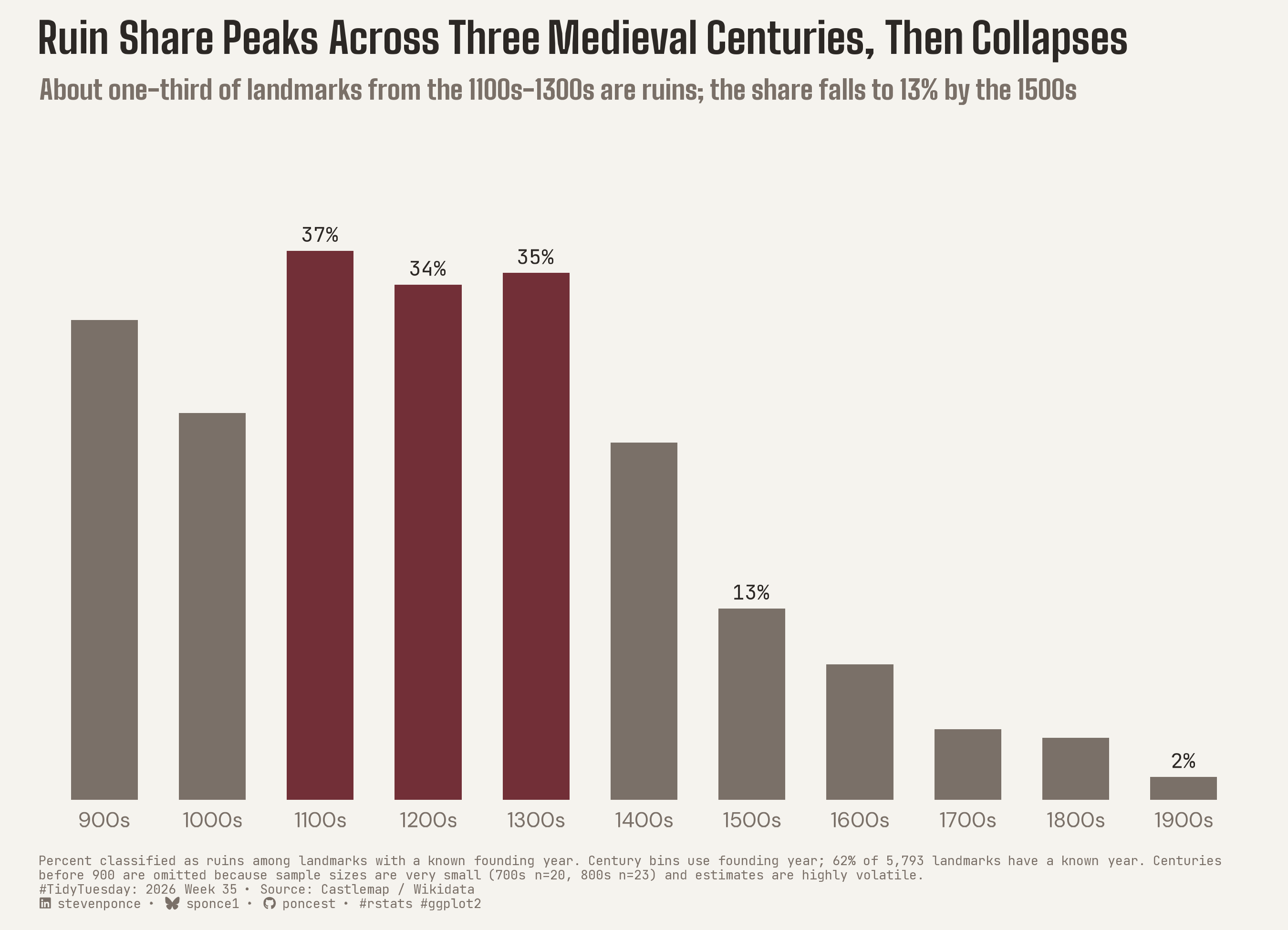
Ruin Share Peaks Across Three Medieval Centuries, Then Collapses

About one-third of landmarks from the 1100s-1300s are ruins; the share falls to 13% by the 1500s

Ruin share among world castles, fortresses, and palaces peaks at roughly 35% across the 1100s-1300s before falling sharply after 1400, reaching just 2% by the 1900s. Century-level founding-year bins were tested for robustness against a coarser seven-era grouping and a country fixed-effects model before being finalized. Built in R with ggplot2, ggtext, and showtext.

Figure 1: Bar chart titled “Ruin Share Peaks Across Three Medieval Centuries, Then Collapses,” showing the percentage of world castles, fortresses, and palaces classified as ruins by century of founding, 900s through 1900s. Ruin share holds near 35 percent across three consecutive centuries — 37% in the 1100s, 34% in the 1200s, 35% in the 1300s — highlighted in burgundy against gray bars for all other centuries. Before this plateau, ruin share was 32% in the 900s and 26% in the 1000s. After it, ruin share falls steadily: 24% in the 1400s, 13% in the 1500s, 9% in the 1600s, 5% in the 1700s, 4% in the 1800s, and 2% in the 1900s. Centuries before 900 are excluded due to small, volatile sample sizes. Data from Castlemap and Wikidata, restricted to landmarks with a known founding year.

Steps to Create this Graphic

1. Load Packages & Setup

```{r}
#| label: load
#| warning: false
#| message: false      
#| results: "hide"     

## 1. LOAD PACKAGES & SETUP ----
suppressPackageStartupMessages({
if (!require("pacman")) install.packages("pacman")
pacman::p_load(
    tidyverse, ggtext, showtext, janitor, ggrepel,      
    scales, glue, skimr, ggview
    )
})

# Source utility functions
suppressMessages(source(here::here("R/utils/fonts.R")))
source(here::here("R/utils/social_icons.R"))
source(here::here("R/utils/image_utils.R"))
source(here::here("R/themes/base_theme.R"))
```

2. Read in the Data

```{r}
#| label: read
#| include: true
#| eval: true
#| warning: false

## 2. READ IN THE DATA ----
# tt <- tidytuesdayR::tt_load(2026, week = 35)
# world_castles <- tt$world_castles
# rm(tt)
world_castles <- readr::read_csv('https://raw.githubusercontent.com/rfordatascience/tidytuesday/main/data/2026/2026-09-01/world_castles.csv')
```

3. Examine the Data

```{r}
#| label: examine
#| include: true
#| eval: true
#| results: 'hide'
#| warning: false

## 3. EXAMINING THE DATA ----
glimpse(world_castles)
skim_without_charts(world_castles)
```

4. Tidy Data

```{r}
#| label: tidy
#| warning: false

### |- century-level ruin share ----
ruin_by_century <- world_castles |>
  filter(!is.na(year)) |>
  mutate(
    century_bin = floor(year / 100) * 100,
    is_ruin = category == "ruin"
  ) |>
  summarise(
    n = n(),
    ruins = sum(is_ruin),
    ruin_share = mean(is_ruin),
    .by = century_bin
  ) |>
  arrange(century_bin)

### |- restrict to the defensible analytical window ----
plot_data <- ruin_by_century |>
  filter(century_bin >= 900, century_bin <= 1900) |>
  mutate(
    century_label = str_glue("{century_bin}s"),
    tier = if_else(century_bin %in% c(1100, 1200, 1300), "plateau", "main"),
    tier = factor(tier, levels = c("main", "plateau")),
    label_text = if_else(
      century_bin %in% c(1100, 1200, 1300, 1500, 1900),
      scales::percent(ruin_share, accuracy = 1),
      NA_character_
    )
  )

### |- known-year denominator, for caption ----
n_known_year <- sum(!is.na(world_castles$year))
n_total <- nrow(world_castles)
pct_known <- scales::percent(n_known_year / n_total, accuracy = 1)
```

5. Visualization Parameters

```{r}
#| label: params
#| include: true
#| warning: false

### |-  plot aesthetics ----
clrs <- get_theme_colors(
  palette = c(
    plateau = "#722F37",
    main    = "#7A7068"
  )
)

col_plateau <- "#722F37"
col_main <- "#7A7068"
col_ink <- "#2C2825"
col_stone <- "#7A7068"

fill_palette <- c(plateau = col_plateau, main = col_main)

### |- fonts ----
setup_fonts()
fonts <- get_font_families()

### |- titles and caption ----
title_text <- str_glue("Ruin Share Peaks Across Three Medieval Centuries, Then Collapses")

subtitle_text <- str_glue(
  "About one-third of landmarks from the 1100s-1300s are ruins; ",
  "the share falls to 13% by the 1500s"
)

methodology_text <- str_glue(
  "Percent classified as ruins among landmarks with a known founding year. ",
  "Century bins use founding year; {pct_known} of {comma(n_total)} landmarks have a known year. ",
  "Centuries before 900 are omitted because sample sizes are very small ",
  "(700s n=20, 800s n=23) and estimates are highly volatile."
)

caption_text <- str_glue(
  "{methodology_text}<br>",
  create_social_caption(
    tt_year = 2026,
    tt_week = 35,
    source_text = "Castlemap / Wikidata"
  )
)

### |- plot theme ----
base_theme <- create_base_theme(clrs)

weekly_theme <- extend_weekly_theme(
  base_theme,
  theme(
    plot.title = element_textbox_simple(
      size = 20,
      face = "bold",
      family = fonts$title_1,
      color = col_ink,
      lineheight = 1.1,
      margin = margin(b = 8)
    ),
    plot.subtitle = element_text(
      size = 12.5,
      family = fonts$title_1,
      color = col_stone,
      margin = margin(b = 16)
    ),
    plot.caption = element_textbox_simple(
      size = 6.0,
      family = fonts$caption,
      color = col_stone,
      margin = margin(t = 12)
    ),
    panel.grid.major.y = element_blank(),
    panel.grid.major.x = element_blank(),
    panel.grid.minor = element_blank(),
    axis.ticks = element_blank(),
    axis.text.x = element_text(size = 10, family = fonts$text),
    axis.text.y = element_blank(),
    axis.title = element_blank(),
    legend.position = "none"
  )
)

theme_set(weekly_theme)
```

6. Plot

```{r}
#| label: plot
#| warning: false

### |-  plot ----
p <- ggplot(plot_data, aes(x = century_label, y = ruin_share, fill = tier)) +
    geom_col(width = 0.62) +
    geom_text(
        aes(label = label_text),
        vjust = -0.6,
        size = 3.4,
        family = fonts$caption,
        color = col_ink,
        na.rm = TRUE
    ) +
    scale_x_discrete(
        limits = plot_data$century_label
    ) +
    scale_y_continuous(
        limits = c(0, 0.42),
        expand = expansion(mult = c(0, 0.05)),
        labels = scales::percent_format(accuracy = 1)
    ) +
    scale_fill_manual(values = fill_palette) +
    labs(
        title = title_text,
        subtitle = subtitle_text,
        caption = caption_text
    )
```

7. Save

```{r}
#| label: save
#| warning: false

### |- save ----
main_path  <- here::here("data_visualizations", "TidyTuesday", "2026", "tt_2026_35.png")
thumb_path <- here::here("data_visualizations", "TidyTuesday", "2026", "thumbnails", "tt_2026_35.png")

# Full-size version, for the QMD figure
save_ggplot(
  plot = p,
  file = main_path,
  width = 9,
  height = 6.5,
  units = "in",
  dpi = 300,
  create.dir = TRUE
)

# Reduced-size thumbnail, for the YAML `image:` field
fs::dir_create(dirname(thumb_path))
magick::image_read(main_path) |>
  magick::image_resize("400") |>
  magick::image_write(thumb_path)
```

8. Session Info

TipExpand for Session Info

R version 4.6.1 (2026-06-24)
Platform: aarch64-apple-darwin23
Running under: macOS Tahoe 26.6.2

Matrix products: default
BLAS:   /Library/Frameworks/R.framework/Versions/4.6/Resources/lib/libRblas.0.dylib 
LAPACK: /Library/Frameworks/R.framework/Versions/4.6/Resources/lib/libRlapack.dylib;  LAPACK version 3.12.1

locale:
[1] en_US.UTF-8/en_US.UTF-8/en_US.UTF-8/C/en_US.UTF-8/en_US.UTF-8

time zone: America/New_York
tzcode source: internal

attached base packages:
[1] stats     graphics  grDevices utils     datasets  methods   base     

other attached packages:
 [1] here_1.0.2      ggview_0.2.2    skimr_2.2.2     glue_1.8.1     
 [5] scales_1.4.0    ggrepel_0.9.8   janitor_2.2.1   showtext_0.9-8 
 [9] showtextdb_3.0  sysfonts_0.8.9  ggtext_0.1.2    lubridate_1.9.5
[13] forcats_1.0.1   stringr_1.6.0   dplyr_1.2.1     purrr_1.2.2    
[17] readr_2.2.0     tidyr_1.3.2     tibble_3.3.1    ggplot2_4.0.3  
[21] tidyverse_2.0.0 pacman_0.5.1   

loaded via a namespace (and not attached):
 [1] gtable_0.3.6       xfun_0.60          htmlwidgets_1.6.4  tzdb_0.5.0        
 [5] vctrs_0.7.3        tools_4.6.1        generics_0.1.4     curl_7.1.0        
 [9] parallel_4.6.1     pkgconfig_2.0.3    RColorBrewer_1.1-3 S7_0.2.2          
[13] lifecycle_1.0.5    compiler_4.6.1     farver_2.1.2       textshaping_1.0.5 
[17] repr_1.1.7         codetools_0.2-20   snakecase_0.11.1   litedown_0.10     
[21] htmltools_0.5.9    yaml_2.3.12        pillar_1.11.1      crayon_1.5.3      
[25] magick_2.9.1       commonmark_2.0.0   tidyselect_1.2.1   digest_0.6.39     
[29] stringi_1.8.7      labeling_0.4.3     rprojroot_2.1.1    fastmap_1.2.0     
[33] grid_4.6.1         cli_3.6.6          magrittr_2.0.5     base64enc_0.1-6   
[37] withr_3.0.3        bit64_4.8.2        timechange_0.4.0   rmarkdown_2.31    
[41] bit_4.6.0          otel_0.2.0         ragg_1.5.2         hms_1.1.4         
[45] evaluate_1.0.5     knitr_1.51         markdown_2.0       rlang_1.3.0       
[49] gridtext_0.1.6     Rcpp_1.1.2         xml2_1.6.0         rstudioapi_0.19.0 
[53] vroom_1.7.1        jsonlite_2.0.0     R6_2.6.1           fs_2.1.0          
[57] systemfonts_1.3.2 

9. GitHub Repository

TipExpand for GitHub Repo

The complete code for this analysis is available in tt_2026_35.qmd.

For the full repository, click here.

10. References

TipExpand for References

1. Data Source:
   • TidyTuesday 2026 Week 35: World Castles, Fortresses and Palaces

11. Custom Functions Documentation

Note📦 Custom Helper Functions

This analysis uses custom functions from my personal module library for efficiency and consistency across projects.

Functions Used:

• fonts.R: setup_fonts(), get_font_families() - Font management with showtext
• social_icons.R: create_social_caption() - Generates formatted social media captions
• image_utils.R: save_plot() - Consistent plot saving with naming conventions
• base_theme.R: create_base_theme(), extend_weekly_theme(), get_theme_colors() - Custom ggplot2 themes

Why custom functions?
These utilities standardize theming, fonts, and output across all my data visualizations. The core analysis (data tidying and visualization logic) uses only standard tidyverse packages.

Source Code:
View all custom functions → GitHub: R/utils