Steven Ponce
  • About
  • Data Visualizations
  • Behind the Viz
  • Projects
  • Resume
  • Email

On this page

  • Steps to Create this Graphic
    • 1. Load Packages & Setup
    • 2. Read in the Data
    • 3. Examine the Data
    • 4. Tidy Data
    • 5. Visualization Parameters
    • 6. Plot
  • 7. Save
    • 8. Session Info
    • 9. GitHub Repository
    • 10. References
    • 11. Custom Functions Documentation

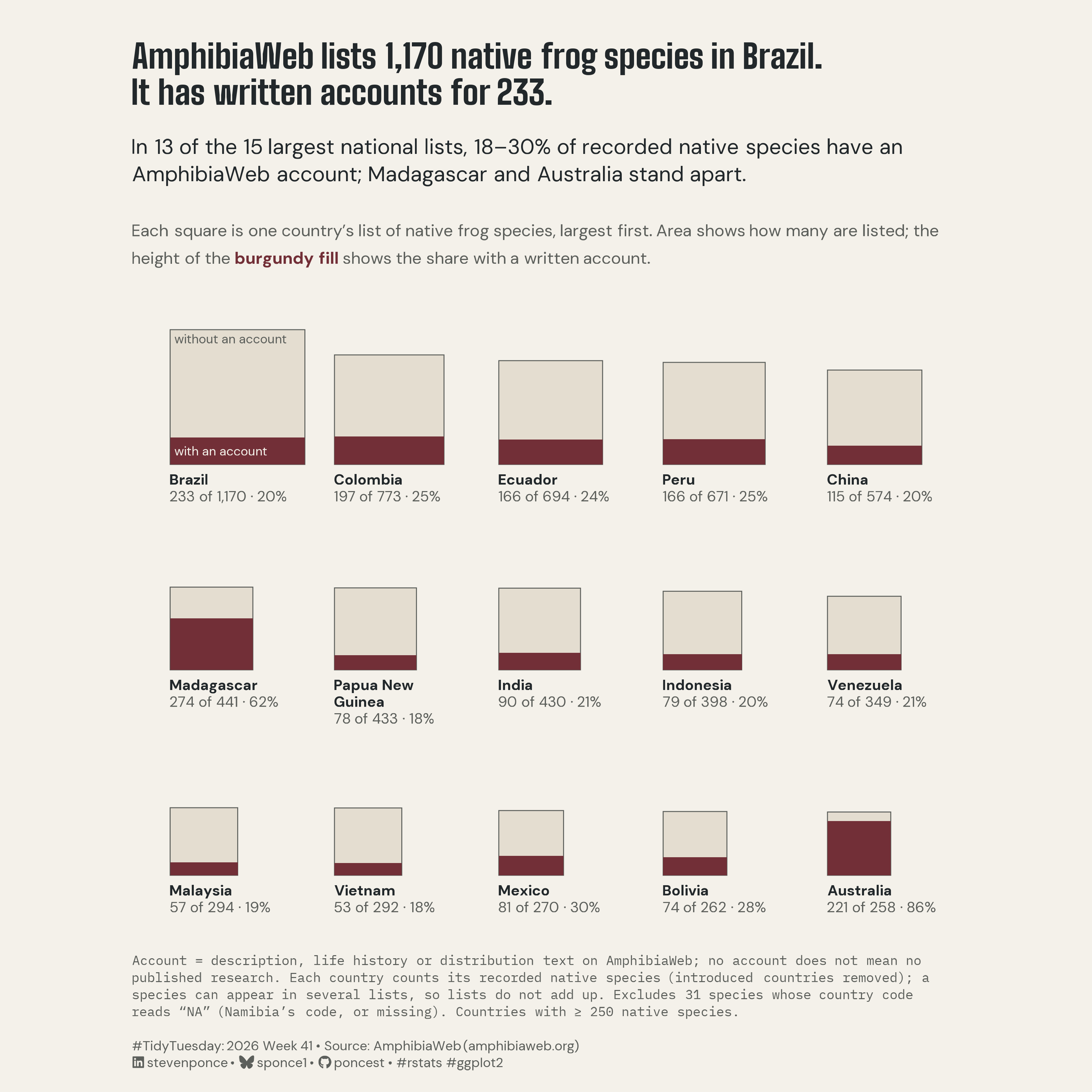
AmphibiaWeb lists 1,170 native frog species in Brazil. It has written accounts for 233.

  • Show All Code
  • Hide All Code

  • View Source

In 13 of the 15 largest national lists, 18–30% of recorded native species have an AmphibiaWeb account; Madagascar and Australia stand apart.

TidyTuesday
2026
Fill-level squares show that AmphibiaWeb has written accounts for 233 of Brazil’s 1,170 native frog species, and for 18–30% of species in 13 of the 15 largest national lists. Native lists exclude introduced countries and ambiguous country codes, and a species counts in every country where it occurs. Built in R with ggplot2, ggtext and showtext.
Author

Steven Ponce

Published

October 12, 2026

Figure 1: AmphibiaWeb has written accounts for 233 of the 1,170 native frog species it lists for Brazil (20%). A 15-square grid, one per country with at least 250 native species, runs from the largest list to the smallest; each square’s area shows the number of native species, and a burgundy fill rising from the bottom shows the share with an account. In 13 of the 15 countries, the share sits between 18% and 30%; Madagascar (274 of 441, 62%) and Australia (221 of 258, 86%) stand apart. An account means a description, life-history, or distribution text on AmphibiaWeb; a missing account does not mean a species lacks published research. Species found in several countries count in each list, so lists cannot be added together. Introduced occurrences and 31 species with ambiguous country codes are excluded. Source: AmphibiaWeb via TidyTuesday 2026 week 41.

Steps to Create this Graphic

1. Load Packages & Setup

Show code
```{r}
#| label: load
#| warning: false
#| message: false      
#| results: "hide"     

## 1. LOAD PACKAGES & SETUP ----
suppressPackageStartupMessages({
if (!require("pacman")) install.packages("pacman")
pacman::p_load(
    tidyverse, ggtext, showtext, janitor, scales, 
    glue, ggview, magick, countrycode
    )
})

# Source utility functions
suppressMessages(source(here::here("R/utils/fonts.R")))
source(here::here("R/utils/social_icons.R"))
source(here::here("R/utils/image_utils.R"))
source(here::here("R/themes/base_theme.R"))
```

2. Read in the Data

Show code
```{r}
#| label: read
#| include: true
#| eval: true
#| warning: false

### |- figure settings ----
fig_w <- 10
fig_h <- 10

## 2. READ IN THE DATA ----
url <- "https://raw.githubusercontent.com/rfordatascience/tidytuesday/main/data/2026/2026-10-13/frogs_and_toads_amphibiaweb.csv"

frogs_raw <- readr::read_csv(
  url,
  col_types = cols(.default = col_character()),
  na = character()
) |>
  clean_names()
```

3. Examine the Data

Show code
```{r}
#| label: examine
#| include: true
#| eval: true
#| results: 'hide'
#| warning: false

## 3. EXAMINING THE DATA ----
glimpse(frogs_raw)
skimr::skim(frogs_raw)
```

4. Tidy Data

Show code
```{r}
#| label: tidy
#| warning: false

frogs <- frogs_raw |>
  mutate(
    across(-c(isocc, intro_isocc), \(x) na_if(x, "NA")),
    intro_isocc = na_if(intro_isocc, "NA"),
    has_account = !is.na(description) | !is.na(life_history) | !is.na(distribution)
  )

intro <- frogs |>
  filter(!is.na(intro_isocc)) |>
  transmute(amphib_id, cc = str_split(str_remove_all(intro_isocc, " "), ",")) |>
  unnest(cc) |>
  filter(cc != "") |>
  mutate(introduced = TRUE)

native <- frogs |>
  filter(isocc != "NA") |>
  select(amphib_id, has_account, isocc) |>
  mutate(cc = str_split(str_remove_all(isocc, " "), ",")) |>
  unnest(cc) |>
  filter(cc != "") |>
  left_join(intro, by = c("amphib_id", "cc")) |>
  filter(is.na(introduced)) |>
  distinct(amphib_id, cc, has_account)

country <- native |>
  summarise(n = n_distinct(amphib_id), written = sum(has_account), .by = cc) |>
  mutate(
    share = written / n,
    pct = round(100 * share),
    name = countrycode(cc, "iso2c", "country.name", warn = FALSE)
  ) |>
  arrange(desc(n))

min_species <- 250
grid15 <- country |> filter(n >= min_species)

n_ambiguous <- sum(frogs$isocc == "NA")
br <- grid15 |> filter(cc == "BR")

## the 13-country band and the two exceptions
band <- grid15 |> filter(pct <= 30)
exceptions <- grid15 |>
  filter(pct > 30) |>
  arrange(desc(n))
band_rng <- range(band$pct)
```

5. Visualization Parameters

Show code
```{r}
#| label: params
#| include: true
#| warning: false

### |-  plot aesthetics ----
col_paper <- "#f4f1ea"
col_ink <- "#22282b"
col_soft <- "#5c5f5b"
col_rest <- "#e4ddd0"
col_accent <- "#722F37"

clrs <- get_theme_colors(
  palette = list(paper = col_paper, ink = col_ink, soft = col_soft, accent = col_accent)
)

### |-  fonts ----
setup_fonts()
fonts <- get_font_families()
if (!"IBM Plex Mono" %in% sysfonts::font_families()) {
    sysfonts::font_add_google("IBM Plex Mono", "IBM Plex Mono")
}
title_family <- fonts$title_1          
text_family  <- fonts$text         
mono_family  <- "IBM Plex Mono"

### |- titles and caption ----
title_text <- glue(
  "AmphibiaWeb lists {comma(br$n)} native frog species in {br$name}.<br>",
  "It has written accounts for {comma(br$written)}."
)

subtitle_text <- glue(
  "In {nrow(band)} of the {nrow(grid15)} largest national lists, ",
  "{band_rng[1]}–{band_rng[2]}% of recorded native species have an ",
  "AmphibiaWeb account; {exceptions$name[1]} and {exceptions$name[2]} stand apart.",
  "<br><br>",
  "<span style='font-size:11pt; color:{col_soft}'>Each square is one country's list ",
  "of native frog species, largest first. Area shows how many are listed; the ",
  "height of the <b style='color:{col_accent}'>burgundy fill</b> shows the share ",
  "with a written account.</span>"
)

method_note <- glue(
  "Account = description, life history or distribution text on AmphibiaWeb; ",
  "no account does not mean no published research. Each country counts its ",
  "recorded native species (introduced countries removed); a species can appear ",
  "in several lists, so lists do not add up. Excludes {n_ambiguous} species whose ",
  "country code reads \"NA\" (Namibia's code, or missing). Countries with ",
  "≥ {min_species} native species."
)

social <- create_social_caption(
  tt_year = 2026,
  tt_week = 41,
  source_text = "AmphibiaWeb (amphibiaweb.org)"
)
caption_text <- glue(
  "<span style='font-family:\"{mono_family}\"'>{method_note}</span><br><br>{social}"
)

## Layout: one cell per country, 5 x 3.
grid_cols <- 5
row_step <- 1.25
max_side <- 0.82

squares <- grid15 |>
  arrange(desc(n)) |>
  mutate(
    i = row_number() - 1,
    x0 = i %% grid_cols,
    y0 = -(i %/% grid_cols) * row_step,
    name_lab = if_else(nchar(name) > 13, str_replace(name, " (?=\\S+$)", "<br>"), name),
    side = sqrt(n / max(n)) * max_side, # outer AREA proportional to n
    level = side * share, # band HEIGHT proportional to share
    label = glue(
      "<b>{name_lab}</b><br>",
      "<span style='color:{col_soft}'>{written} of {comma(n)} · {pct}%</span>"
    )
  )

# Brazil teaches the encoding once, in words only (its numbers sit below).
br_sq <- squares |> filter(cc == "BR")

key_labels <- tibble(
  x      = br_sq$x0 + 0.025,
  y      = c(br_sq$y0 + br_sq$side - 0.03, br_sq$y0 + br_sq$level / 2),
  label  = c("without an account", "with an account"),
  color = c(col_soft, col_paper),
  vjust  = c(1, 0.5)
)

### |-  plot theme ----
base_theme <- create_base_theme(clrs)

weekly_theme <- extend_weekly_theme(
  base_theme,
  theme(
    plot.background = element_rect(fill = col_paper, color = NA),
    panel.background = element_rect(fill = col_paper, color = NA),
    panel.grid = element_blank(),
    axis.text = element_blank(),
    axis.title = element_blank(),
    axis.ticks = element_blank(),
    plot.title = element_textbox_simple(
      family = title_family, color = col_ink, size = rel(1.55),
      lineheight = 1.1, margin = margin(b = 18)
    ),
    plot.subtitle = element_textbox_simple(
      family = text_family, color = col_ink, size = rel(1.0),
      lineheight = 1.3, margin = margin(b = 22)
    ),
    plot.caption = element_textbox_simple(
      family = text_family, color = col_soft, size = rel(0.62),
      lineheight = 1.3, margin = margin(t = 34)
    ),
    plot.title.position = "plot",
    plot.caption.position = "plot",
    plot.margin = margin(28, 32, 20, 32)
  )
)

theme_set(weekly_theme)
```

6. Plot

Show code
```{r}
#| label: plot
#| warning: false

### |-  main plot ----
p <- ggplot(squares) +
    geom_rect(aes(xmin = x0, xmax = x0 + side, ymin = y0, ymax = y0 + side),
      fill = col_rest, color = col_soft, linewidth = 0.3
    ) +
      geom_rect(aes(xmin = x0, xmax = x0 + side, ymin = y0, ymax = y0 + level),
        fill = col_accent, color = NA
      ) +
      geom_text(
        data = key_labels,
        aes(x = x, y = y, label = label, color = color, vjust = vjust),
        hjust = 0, size = 2.9, family = text_family
      ) + 
      scale_color_identity() +
      geom_richtext(aes(x = x0, y = y0 - 0.06, label = label),
        hjust = 0, vjust = 1, size = 3.4, lineheight = 1.15,
        family = text_family, color = col_ink,
        fill = NA, label.color = NA, label.padding = unit(0, "pt")
      ) +
      coord_equal(clip = "off") +
      labs(title = title_text, subtitle = subtitle_text, caption = caption_text)
```

7. Save

Show code
```{r}
#| label: save
#| warning: false

### |- save ----
main_path  <- here::here("data_visualizations", "TidyTuesday", "2026", "tt_2026_41.png")
thumb_path <- here::here("data_visualizations", "TidyTuesday", "2026", "thumbnails", "tt_2026_41.png")

# Full-size version, for the QMD figure
ggview::save_ggplot(
    plot   = p,
    file   = main_path,
    width  = fig_w,
    height = fig_h,
    units  = "in",
    dpi    = 320
)

# Reduced-size thumbnail, for the YAML `image:` field
fs::dir_create(dirname(thumb_path))
magick::image_read(main_path) |>
  magick::image_resize("400") |>
  magick::image_write(thumb_path)
```

8. Session Info

TipExpand for Session Info
R version 4.6.1 (2026-06-24)
Platform: aarch64-apple-darwin23
Running under: macOS Tahoe 26.6.2

Matrix products: default
BLAS:   /Library/Frameworks/R.framework/Versions/4.6/Resources/lib/libRblas.0.dylib 
LAPACK: /Library/Frameworks/R.framework/Versions/4.6/Resources/lib/libRlapack.dylib;  LAPACK version 3.12.1

locale:
[1] en_US.UTF-8/en_US.UTF-8/en_US.UTF-8/C/en_US.UTF-8/en_US.UTF-8

time zone: America/New_York
tzcode source: internal

attached base packages:
[1] stats     graphics  grDevices utils     datasets  methods   base     

other attached packages:
 [1] here_1.0.2        countrycode_1.9.0 magick_2.9.1      ggview_0.2.2     
 [5] glue_1.8.1        scales_1.4.0      janitor_2.2.1     showtext_0.9-8   
 [9] showtextdb_3.0    sysfonts_0.8.9    ggtext_0.2.0      lubridate_1.9.5  
[13] forcats_1.0.1     stringr_1.6.0     dplyr_1.2.1       purrr_1.2.2      
[17] readr_2.2.0       tidyr_1.3.2       tibble_3.3.1      ggplot2_4.0.3    
[21] tidyverse_2.0.0   pacman_0.5.1     

loaded via a namespace (and not attached):
 [1] gtable_0.3.6       xfun_0.60          htmlwidgets_1.6.4  tzdb_0.5.0        
 [5] vctrs_0.7.3        tools_4.6.1        generics_0.1.4     curl_7.1.0        
 [9] parallel_4.6.1     pkgconfig_2.0.3    RColorBrewer_1.1-3 skimr_2.2.2       
[13] S7_0.2.2           lifecycle_1.0.5    compiler_4.6.1     farver_2.1.2      
[17] textshaping_1.0.5  repr_1.1.7         codetools_0.2-20   snakecase_0.11.1  
[21] litedown_0.10      htmltools_0.5.9    yaml_2.3.12        pillar_1.11.1     
[25] crayon_1.5.3       commonmark_2.0.0   tidyselect_1.2.1   digest_0.6.39     
[29] stringi_1.8.7      labeling_0.4.3     rprojroot_2.1.1    fastmap_1.2.0     
[33] grid_4.6.1         cli_3.6.6          magrittr_2.0.5     base64enc_0.1-6   
[37] withr_3.0.3        bit64_4.8.2        timechange_0.4.0   rmarkdown_2.31    
[41] bit_4.6.0          otel_0.2.0         ragg_1.5.2         hms_1.1.4         
[45] evaluate_1.0.5     knitr_1.51         markdown_2.0       rlang_1.3.0       
[49] gridtext_0.1.6     Rcpp_1.1.2         xml2_1.6.0         rstudioapi_0.19.0 
[53] vroom_1.7.1        jsonlite_2.0.0     R6_2.6.1           fs_2.1.0          
[57] systemfonts_1.3.2 

9. GitHub Repository

TipExpand for GitHub Repo

The complete code for this analysis is available in tt_2026_41.qmd.

For the full repository, click here.

10. References

TipExpand for References
  1. Data Source:
    • TidyTuesday 2026 Week 41: AmphibiaWeb

11. Custom Functions Documentation

Note📦 Custom Helper Functions

This analysis uses custom functions from my personal module library for efficiency and consistency across projects.

Functions Used:

  • fonts.R: setup_fonts(), get_font_families() - Font management with showtext
  • social_icons.R: create_social_caption() - Generates formatted social media captions
  • image_utils.R: save_plot() - Consistent plot saving with naming conventions
  • base_theme.R: create_base_theme(), extend_weekly_theme(), get_theme_colors() - Custom ggplot2 themes

Why custom functions?
These utilities standardize theming, fonts, and output across all my data visualizations. The core analysis (data tidying and visualization logic) uses only standard tidyverse packages.

Source Code:
View all custom functions → GitHub: R/utils

Back to top

Citation

BibTeX citation:
@online{ponce2026,
  author = {Ponce, Steven},
  title = {AmphibiaWeb Lists 1,170 Native Frog Species in {Brazil.} {It}
    Has Written Accounts for 233.},
  date = {2026-10-12},
  url = {https://stevenponce.netlify.app/data_visualizations/TidyTuesday/2026/tt_2026_41.html},
  langid = {en}
}
For attribution, please cite this work as:
Ponce, Steven. 2026. “AmphibiaWeb Lists 1,170 Native Frog Species in Brazil. It Has Written Accounts for 233.” October 12. https://stevenponce.netlify.app/data_visualizations/TidyTuesday/2026/tt_2026_41.html.
Source Code
---
title: "AmphibiaWeb lists 1,170 native frog species in Brazil. It has written accounts for 233."
subtitle: "In 13 of the 15 largest national lists, 18–30% of recorded native species have an AmphibiaWeb account; Madagascar and Australia stand apart."
description: "Fill-level squares show that AmphibiaWeb has written accounts for 233 of Brazil's 1,170 native frog species, and for 18–30% of species in 13 of the 15 largest national lists. Native lists exclude introduced countries and ambiguous country codes, and a species counts in every country where it occurs. Built in R with ggplot2, ggtext and showtext."
date: "2026-10-12"
author:
  - name: "Steven Ponce"
    url: "https://stevenponce.netlify.app"
citation:
  url: "https://stevenponce.netlify.app/data_visualizations/TidyTuesday/2026/tt_2026_41.html"
categories: ["TidyTuesday", "2026"]
tags: [
  "TidyTuesday",
  "AmphibiaWeb",
  "Amphibians",
  "Frogs",
  "Biodiversity",
  "Data Coverage",
  "Proportional Squares",
  "Part-to-Whole",
  "Small Multiples",
  "Country Comparison",
  "ggtext",
  "showtext",
  "ggplot2",
  "2026"
]
image: "thumbnails/tt_2026_41.png"
format:
  html:
    toc: true
    toc-depth: 5
    code-link: true
    code-fold: true
    code-tools: true
    code-summary: "Show code"
editor_options: 
  chunk_output_type: inline
execute: 
  freeze: true
  cache: true
  error: false
  message: false
  warning: false
  eval: true
---
![AmphibiaWeb has written accounts for 233 of the 1,170 native frog species it lists for Brazil (20%). A 15-square grid, one per country with at least 250 native species, runs from the largest list to the smallest; each square's area shows the number of native species, and a burgundy fill rising from the bottom shows the share with an account. In 13 of the 15 countries, the share sits between 18% and 30%; Madagascar (274 of 441, 62%) and Australia (221 of 258, 86%) stand apart. An account means a description, life-history, or distribution text on AmphibiaWeb; a missing account does not mean a species lacks published research. Species found in several countries count in each list, so lists cannot be added together. Introduced occurrences and 31 species with ambiguous country codes are excluded. Source: AmphibiaWeb via TidyTuesday 2026 week 41.](tt_2026_41.png){#fig-1}

### [**Steps to Create this Graphic**]{.mark}

#### [1. Load Packages & Setup]{.smallcaps}

```{r}
#| label: load
#| warning: false
#| message: false      
#| results: "hide"     

## 1. LOAD PACKAGES & SETUP ----
suppressPackageStartupMessages({
if (!require("pacman")) install.packages("pacman")
pacman::p_load(
    tidyverse, ggtext, showtext, janitor, scales, 
    glue, ggview, magick, countrycode
    )
})

# Source utility functions
suppressMessages(source(here::here("R/utils/fonts.R")))
source(here::here("R/utils/social_icons.R"))
source(here::here("R/utils/image_utils.R"))
source(here::here("R/themes/base_theme.R"))
```

#### [2. Read in the Data]{.smallcaps}

```{r}
#| label: read
#| include: true
#| eval: true
#| warning: false

### |- figure settings ----
fig_w <- 10
fig_h <- 10

## 2. READ IN THE DATA ----
url <- "https://raw.githubusercontent.com/rfordatascience/tidytuesday/main/data/2026/2026-10-13/frogs_and_toads_amphibiaweb.csv"

frogs_raw <- readr::read_csv(
  url,
  col_types = cols(.default = col_character()),
  na = character()
) |>
  clean_names()
```

#### [3. Examine the Data]{.smallcaps}

```{r}
#| label: examine
#| include: true
#| eval: true
#| results: 'hide'
#| warning: false

## 3. EXAMINING THE DATA ----
glimpse(frogs_raw)
skimr::skim(frogs_raw)
```

#### [4. Tidy Data]{.smallcaps}

```{r}
#| label: tidy
#| warning: false

frogs <- frogs_raw |>
  mutate(
    across(-c(isocc, intro_isocc), \(x) na_if(x, "NA")),
    intro_isocc = na_if(intro_isocc, "NA"),
    has_account = !is.na(description) | !is.na(life_history) | !is.na(distribution)
  )

intro <- frogs |>
  filter(!is.na(intro_isocc)) |>
  transmute(amphib_id, cc = str_split(str_remove_all(intro_isocc, " "), ",")) |>
  unnest(cc) |>
  filter(cc != "") |>
  mutate(introduced = TRUE)

native <- frogs |>
  filter(isocc != "NA") |>
  select(amphib_id, has_account, isocc) |>
  mutate(cc = str_split(str_remove_all(isocc, " "), ",")) |>
  unnest(cc) |>
  filter(cc != "") |>
  left_join(intro, by = c("amphib_id", "cc")) |>
  filter(is.na(introduced)) |>
  distinct(amphib_id, cc, has_account)

country <- native |>
  summarise(n = n_distinct(amphib_id), written = sum(has_account), .by = cc) |>
  mutate(
    share = written / n,
    pct = round(100 * share),
    name = countrycode(cc, "iso2c", "country.name", warn = FALSE)
  ) |>
  arrange(desc(n))

min_species <- 250
grid15 <- country |> filter(n >= min_species)

n_ambiguous <- sum(frogs$isocc == "NA")
br <- grid15 |> filter(cc == "BR")

## the 13-country band and the two exceptions
band <- grid15 |> filter(pct <= 30)
exceptions <- grid15 |>
  filter(pct > 30) |>
  arrange(desc(n))
band_rng <- range(band$pct)
```

#### [5. Visualization Parameters]{.smallcaps}

```{r}
#| label: params
#| include: true
#| warning: false

### |-  plot aesthetics ----
col_paper <- "#f4f1ea"
col_ink <- "#22282b"
col_soft <- "#5c5f5b"
col_rest <- "#e4ddd0"
col_accent <- "#722F37"

clrs <- get_theme_colors(
  palette = list(paper = col_paper, ink = col_ink, soft = col_soft, accent = col_accent)
)

### |-  fonts ----
setup_fonts()
fonts <- get_font_families()
if (!"IBM Plex Mono" %in% sysfonts::font_families()) {
    sysfonts::font_add_google("IBM Plex Mono", "IBM Plex Mono")
}
title_family <- fonts$title_1          
text_family  <- fonts$text         
mono_family  <- "IBM Plex Mono"

### |- titles and caption ----
title_text <- glue(
  "AmphibiaWeb lists {comma(br$n)} native frog species in {br$name}.<br>",
  "It has written accounts for {comma(br$written)}."
)

subtitle_text <- glue(
  "In {nrow(band)} of the {nrow(grid15)} largest national lists, ",
  "{band_rng[1]}–{band_rng[2]}% of recorded native species have an ",
  "AmphibiaWeb account; {exceptions$name[1]} and {exceptions$name[2]} stand apart.",
  "<br><br>",
  "<span style='font-size:11pt; color:{col_soft}'>Each square is one country's list ",
  "of native frog species, largest first. Area shows how many are listed; the ",
  "height of the <b style='color:{col_accent}'>burgundy fill</b> shows the share ",
  "with a written account.</span>"
)

method_note <- glue(
  "Account = description, life history or distribution text on AmphibiaWeb; ",
  "no account does not mean no published research. Each country counts its ",
  "recorded native species (introduced countries removed); a species can appear ",
  "in several lists, so lists do not add up. Excludes {n_ambiguous} species whose ",
  "country code reads \"NA\" (Namibia's code, or missing). Countries with ",
  "≥ {min_species} native species."
)

social <- create_social_caption(
  tt_year = 2026,
  tt_week = 41,
  source_text = "AmphibiaWeb (amphibiaweb.org)"
)
caption_text <- glue(
  "<span style='font-family:\"{mono_family}\"'>{method_note}</span><br><br>{social}"
)

## Layout: one cell per country, 5 x 3.
grid_cols <- 5
row_step <- 1.25
max_side <- 0.82

squares <- grid15 |>
  arrange(desc(n)) |>
  mutate(
    i = row_number() - 1,
    x0 = i %% grid_cols,
    y0 = -(i %/% grid_cols) * row_step,
    name_lab = if_else(nchar(name) > 13, str_replace(name, " (?=\\S+$)", "<br>"), name),
    side = sqrt(n / max(n)) * max_side, # outer AREA proportional to n
    level = side * share, # band HEIGHT proportional to share
    label = glue(
      "<b>{name_lab}</b><br>",
      "<span style='color:{col_soft}'>{written} of {comma(n)} · {pct}%</span>"
    )
  )

# Brazil teaches the encoding once, in words only (its numbers sit below).
br_sq <- squares |> filter(cc == "BR")

key_labels <- tibble(
  x      = br_sq$x0 + 0.025,
  y      = c(br_sq$y0 + br_sq$side - 0.03, br_sq$y0 + br_sq$level / 2),
  label  = c("without an account", "with an account"),
  color = c(col_soft, col_paper),
  vjust  = c(1, 0.5)
)

### |-  plot theme ----
base_theme <- create_base_theme(clrs)

weekly_theme <- extend_weekly_theme(
  base_theme,
  theme(
    plot.background = element_rect(fill = col_paper, color = NA),
    panel.background = element_rect(fill = col_paper, color = NA),
    panel.grid = element_blank(),
    axis.text = element_blank(),
    axis.title = element_blank(),
    axis.ticks = element_blank(),
    plot.title = element_textbox_simple(
      family = title_family, color = col_ink, size = rel(1.55),
      lineheight = 1.1, margin = margin(b = 18)
    ),
    plot.subtitle = element_textbox_simple(
      family = text_family, color = col_ink, size = rel(1.0),
      lineheight = 1.3, margin = margin(b = 22)
    ),
    plot.caption = element_textbox_simple(
      family = text_family, color = col_soft, size = rel(0.62),
      lineheight = 1.3, margin = margin(t = 34)
    ),
    plot.title.position = "plot",
    plot.caption.position = "plot",
    plot.margin = margin(28, 32, 20, 32)
  )
)

theme_set(weekly_theme)

```

#### [6. Plot]{.smallcaps}

```{r}
#| label: plot
#| warning: false

### |-  main plot ----
p <- ggplot(squares) +
    geom_rect(aes(xmin = x0, xmax = x0 + side, ymin = y0, ymax = y0 + side),
      fill = col_rest, color = col_soft, linewidth = 0.3
    ) +
      geom_rect(aes(xmin = x0, xmax = x0 + side, ymin = y0, ymax = y0 + level),
        fill = col_accent, color = NA
      ) +
      geom_text(
        data = key_labels,
        aes(x = x, y = y, label = label, color = color, vjust = vjust),
        hjust = 0, size = 2.9, family = text_family
      ) + 
      scale_color_identity() +
      geom_richtext(aes(x = x0, y = y0 - 0.06, label = label),
        hjust = 0, vjust = 1, size = 3.4, lineheight = 1.15,
        family = text_family, color = col_ink,
        fill = NA, label.color = NA, label.padding = unit(0, "pt")
      ) +
      coord_equal(clip = "off") +
      labs(title = title_text, subtitle = subtitle_text, caption = caption_text)
```

### [7. Save]{.smallcaps}

```{r}
#| label: save
#| warning: false

### |- save ----
main_path  <- here::here("data_visualizations", "TidyTuesday", "2026", "tt_2026_41.png")
thumb_path <- here::here("data_visualizations", "TidyTuesday", "2026", "thumbnails", "tt_2026_41.png")

# Full-size version, for the QMD figure
ggview::save_ggplot(
    plot   = p,
    file   = main_path,
    width  = fig_w,
    height = fig_h,
    units  = "in",
    dpi    = 320
)

# Reduced-size thumbnail, for the YAML `image:` field
fs::dir_create(dirname(thumb_path))
magick::image_read(main_path) |>
  magick::image_resize("400") |>
  magick::image_write(thumb_path)
```


#### [8. Session Info]{.smallcaps}

::: {.callout-tip collapse="true"}
##### Expand for Session Info

```{r, echo = FALSE}
#| eval: true
#| warning: false

sessionInfo()
```
:::

#### [9. GitHub Repository]{.smallcaps}

::: {.callout-tip collapse="true"}
##### Expand for GitHub Repo

The complete code for this analysis is available in [`tt_2026_41.qmd`](https://github.com/poncest/personal-website/blob/master/data_visualizations/TidyTuesday/2026/tt_2026_41.qmd).

For the full repository, [click here](https://github.com/poncest/personal-website/).
:::

#### [10. References]{.smallcaps}

::: {.callout-tip collapse="true"}
##### Expand for References
1.  **Data Source:**
    -   TidyTuesday 2026 Week 41: [AmphibiaWeb](https://github.com/rfordatascience/tidytuesday/blob/main/data/2026/2026-10-13/readme.md)

:::


#### [11. Custom Functions Documentation]{.smallcaps}

::: {.callout-note collapse="true"}
##### 📦 Custom Helper Functions

This analysis uses custom functions from my personal module library for efficiency and consistency across projects.

**Functions Used:**

-   **`fonts.R`**: `setup_fonts()`, `get_font_families()` - Font management with showtext
-   **`social_icons.R`**: `create_social_caption()` - Generates formatted social media captions
-   **`image_utils.R`**: `save_plot()` - Consistent plot saving with naming conventions
-   **`base_theme.R`**: `create_base_theme()`, `extend_weekly_theme()`, `get_theme_colors()` - Custom ggplot2 themes

**Why custom functions?**\
These utilities standardize theming, fonts, and output across all my data visualizations. The core analysis (data tidying and visualization logic) uses only standard tidyverse packages.

**Source Code:**\
View all custom functions → [GitHub: R/utils](https://github.com/poncest/personal-website/tree/master/R)
:::

© 2026 Steven Ponce · Built with R + Quarto

Source Issues