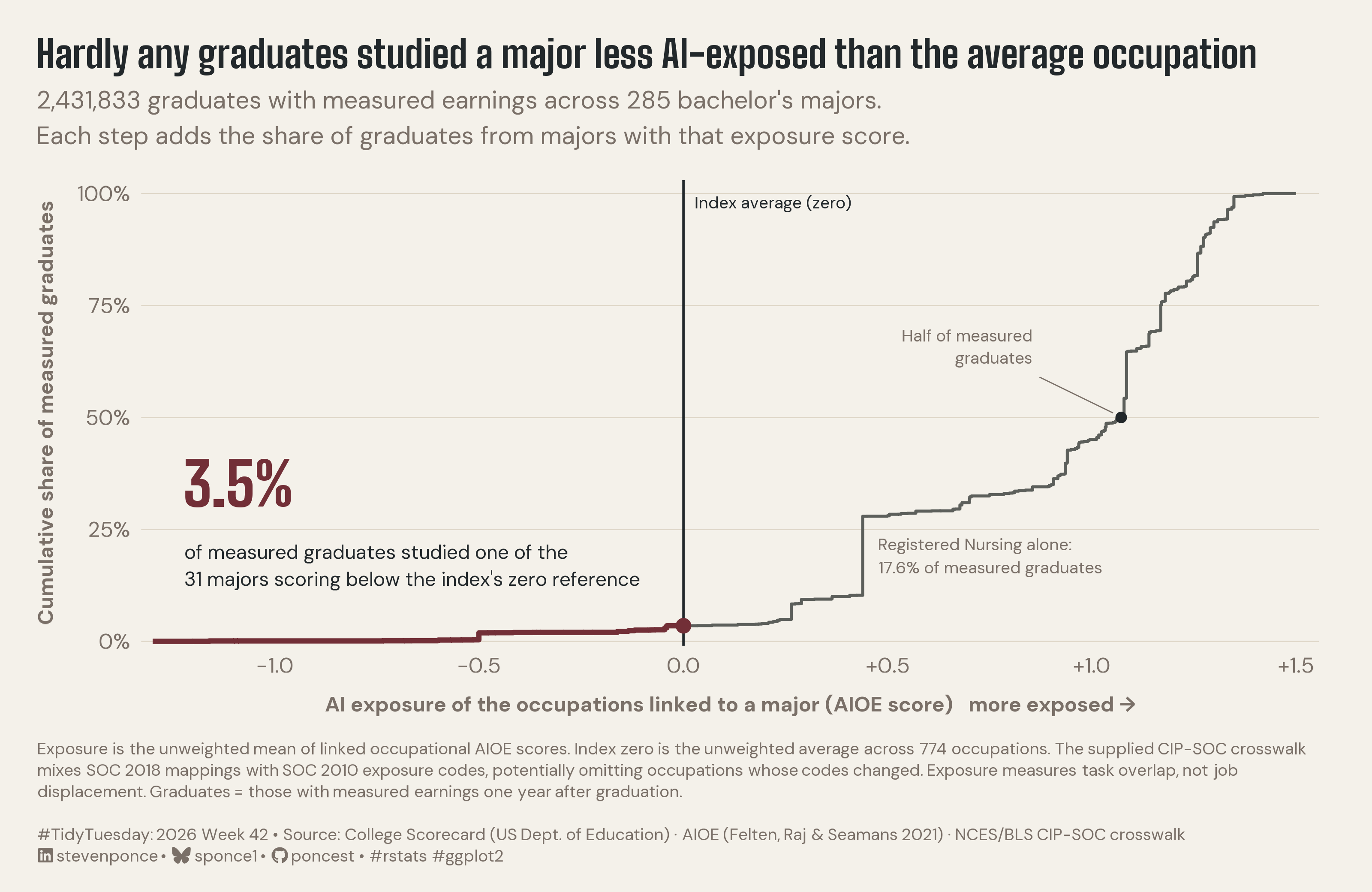
Hardly any graduates studied a major less AI-exposed than the average occupation

2,431,833 graduates with measured earnings across 285 bachelor’s majors. Each step adds the share of graduates from majors with that exposure score.

Only 3.5% of 2.43 million measured graduates studied a major less AI-exposed than the average occupation on the AIOE index. A graduate-weighted cumulative step curve replaces the original chart’s percentile axis with the index’s raw scale. Built in R with ggplot2, ggtext, showtext and ggview.

Figure 1: Cumulative step chart titled “Hardly any graduates studied a major less AI-exposed than the average occupation.” At the index’s zero line, the curve reaches only 3.5%: 3.5% of 2,431,833 graduates with measured earnings studied one of the 31 bachelor’s majors scoring below the average occupation on the AI Occupational Exposure (AIOE) index, highlighted in burgundy. The horizontal axis shows the AIOE score from about −1.3 to +1.5, with zero marking the unweighted average across 774 occupations. The vertical axis shows the cumulative share of measured graduates across 285 majors. To the right of zero, the curve climbs: a single step at +0.44, Registered Nursing, adds 17.6% of graduates, and the curve crosses 50% at about +1.07. Exposure measures overlap with AI abilities, not job displacement. Data: College Scorecard, AIOE (Felten, Raj and Seamans 2021), NCES/BLS CIP-SOC crosswalk.

Steps to Create this Graphic

1. Load Packages & Setup

```{r}
#| label: load
#| warning: false
#| message: false      
#| results: "hide"     

## 1. LOAD PACKAGES & SETUP ----
suppressPackageStartupMessages({
if (!require("pacman")) install.packages("pacman")
pacman::p_load(
    tidyverse, ggtext, showtext, janitor, scales, 
    glue, ggview, magick
    )
})

# Source utility functions
suppressMessages(source(here::here("R/utils/fonts.R")))
source(here::here("R/utils/social_icons.R"))
source(here::here("R/utils/image_utils.R"))
source(here::here("R/themes/base_theme.R"))
```

2. Read in the Data

```{r}
#| label: read
#| include: true
#| eval: true
#| warning: false

### |- figure settings ----
fig_w   <- 10
fig_h   <- 6.5
fig_dpi <- 320
out_file   <- "2026/Week_42/2026_42.png"

setup_fonts()
fonts <- get_font_families()
title_family <- fonts$title_1 %||% fonts$title
text_family  <- fonts$text


## 2. READ IN THE DATA ----
tt <- tidytuesdayR::tt_load(2026, week = 42)
majors_raw <- tt$ai_salary_majors |> clean_names()
rm(tt)
```

3. Examine the Data

```{r}
#| label: examine
#| include: true
#| eval: true
#| results: 'hide'
#| warning: false

## 3. EXAMINING THE DATA ----
glimpse(majors_raw)
skimr::skim(majors_raw)
```

4. Tidy Data

```{r}
#| label: tidy
#| warning: false

### |- majors ----
majors <- majors_raw |>
  mutate(is_rn = str_detect(field_of_study, "^Registered Nursing"))

### |- weighted ECDF: aggregate tied scores, then one step per distinct score ----
ecdf_df <- majors |>
  summarise(
    grads   = sum(n_graduates),
    n_maj   = n(),
    has_rn  = any(is_rn),
    .by     = ai_exposure
  ) |>
  arrange(ai_exposure) |>
  mutate(
    cum_share  = cumsum(grads) / sum(grads),
    prev_share = lag(cum_share, default = 0)
  )

x_min <- -1.3
x_max <- 1.5

step_df <- bind_rows(
  tibble(ai_exposure = x_min, cum_share = 0),
  ecdf_df |> select(ai_exposure, cum_share),
  tibble(ai_exposure = x_max, cum_share = 1)
) |>
  mutate(side = if_else(ai_exposure < 0, "below", "above"))

# Split the step path at zero so the left segment can carry the accent
share_at_zero <- max(ecdf_df$cum_share[ecdf_df$ai_exposure < 0])
step_below <- bind_rows(
  step_df |> filter(ai_exposure < 0),
  tibble(ai_exposure = 0, cum_share = share_at_zero)
)
step_above <- bind_rows(
  tibble(ai_exposure = 0, cum_share = share_at_zero),
  step_df |> filter(ai_exposure >= 0)
)

### |- reader-facing numbers (computed, guarded next to the copy they feed) ----
total_grads <- sum(majors$n_graduates)
n_majors <- nrow(majors)
n_below_zero <- sum(majors$ai_exposure < 0)
share_below <- sum(majors$n_graduates[majors$ai_exposure < 0]) / total_grads

rn_row <- ecdf_df |> filter(has_rn)
rn_exp <- rn_row$ai_exposure
rn_share <- majors$n_graduates[majors$is_rn] / total_grads

# Graduate-weighted median: first exposure score where cumulative share >= 50%
half_row <- ecdf_df |>
  filter(cum_share >= 0.5) |>
  slice_head(n = 1)
x_half <- half_row$ai_exposure

med_major <- median(majors$ai_exposure) # equal-weight median
```

5. Visualization Parameters

```{r}
#| label: params
#| include: true
#| warning: false

### |- plot aesthetics ----
colors <- get_theme_colors(
  palette = list(
    accent    = "#722F37",
    curve     = "#5c5f5b",
    ink       = "#22282b",
    muted     = "#7A7068",
    paper     = "#f4f1ea"
  )
)
clrs <- colors$palette
if (is.null(clrs$accent)) {
  clrs <- list(
    accent = "#722F37", curve = "#5c5f5b",
    ink = "#22282b", muted = "#7A7068", paper = "#f4f1ea"
  )
}
col_accent <- clrs$accent
col_curve <- clrs$curve
col_ink <- clrs$ink
col_muted <- clrs$muted
col_paper <- clrs$paper

### |- titles and caption ----
title_text <- "Hardly any graduates studied a major less AI-exposed than the average occupation"

subtitle_text <- str_glue(
  "{comma(total_grads)} graduates with measured earnings across {n_majors} bachelor's majors.\n",
  "Each step adds the share of graduates from majors with that exposure score."
)

# Provenance constant (not computed from this dataset): AIOE Data Appendix A
n_aioe_occupations <- 774

note_text <- paste(
  "Exposure is the unweighted mean of linked occupational AIOE scores.",
  glue("Index zero is the unweighted average across {n_aioe_occupations} occupations."),
  "The supplied CIP-SOC crosswalk mixes SOC 2018 mappings with SOC 2010 exposure codes,",
  "potentially omitting occupations whose codes changed.",
  "Exposure measures task overlap, not job displacement.",
  "Graduates = those with measured earnings one year after graduation.<br>"
)

caption_text <- create_social_caption(
  tt_year     = 2026,
  tt_week     = 42,
  source_text = "College Scorecard (US Dept. of Education) · AIOE (Felten, Raj & Seamans 2021) · NCES/BLS CIP-SOC crosswalk"
)
caption_full <- paste0(note_text, "<br>", caption_text)

### |- annotation text (built from guarded values) ----
lab_below_big <- percent(share_below, accuracy = 0.1)
lab_below_small <- glue("of measured graduates studied one of the\n{n_below_zero} majors scoring below the index's zero reference")
lab_rn <- glue("Registered Nursing alone:\n{percent(rn_share, accuracy = 0.1)} of measured graduates")
lab_half <- "Half of measured\ngraduates"
lab_zero <- "Index average (zero)"

### |- copy guards ----
all_copy <- c(title_text, subtitle_text, note_text, lab_below_small, lab_rn, lab_half, lab_zero)

### |- plot theme ----
base_theme <- create_base_theme(colors)

weekly_theme <- extend_weekly_theme(
  base_theme,
  theme(
    plot.background = element_rect(fill = col_paper, color = NA),
    panel.background = element_rect(fill = col_paper, color = NA),
    plot.title = element_text(
      family = title_family, face = "bold", size = rel(1.42),
      color = col_ink, lineheight = 1.05, margin = margin(b = 8)
    ),
    plot.subtitle = element_text(
      family = text_family, size = rel(0.92), color = col_muted,
      lineheight = 1.2, margin = margin(b = 16)
    ),
    plot.caption = element_textbox_simple(
      family = text_family, size = rel(0.62), color = col_muted,
      lineheight = 1.3, width = unit(1, "npc"), margin = margin(t = 14)
    ),
    plot.title.position = "plot",
    plot.caption.position = "plot",
    axis.title.x = element_text(
      family = text_family, color = col_muted,
      size = rel(0.85), margin = margin(t = 10)
    ),
    axis.title.y = element_text(
      family = text_family, color = col_muted,
      size = rel(0.85), margin = margin(r = 10)
    ),
    axis.text = element_text(family = text_family, color = col_muted, size = rel(0.8)),
    axis.ticks = element_blank(),
    panel.grid.major.y = element_line(color = "#ddd5c6", linewidth = 0.3),
    panel.grid.major.x = element_blank(),
    panel.grid.minor = element_blank(),
    legend.position = "none",
    plot.margin = margin(20, 28, 14, 20)
  )
)

theme_set(weekly_theme)
```

6. Plot

```{r}
#| label: plot
#| warning: false

### |- annotation positions ----
pos <- list(
  below_x = -1.22, below_big_y = 0.30, below_small_y = 0.215,
  below_pt_x = 0, below_pt_y = share_below,
  rn_x = rn_exp + 0.04, rn_y = (rn_row$prev_share + rn_row$cum_share) / 2, # right of its riser, below the plateau
  half_x = x_half, half_lab_x = x_half - 0.22, half_lab_y = 0.62,
  zero_lab_y = 0.98
)

### |-  main plot ----
p <- ggplot() +
  geom_vline(xintercept = 0, color = col_ink, linewidth = 0.6) +
  geom_step(
    data = step_above, aes(ai_exposure, cum_share),
    direction = "hv", color = col_curve, linewidth = 0.75
  ) +
  geom_step(
    data = step_below, aes(ai_exposure, cum_share),
    direction = "hv", color = col_accent, linewidth = 1.3
  ) +
  annotate("point",
    x = pos$below_pt_x, y = pos$below_pt_y,
    color = col_accent, size = 3
  ) +
  annotate("text",
    x = pos$below_x, y = pos$below_big_y, label = lab_below_big,
    family = title_family, fontface = "bold", size = 11,
    color = col_accent, hjust = 0, vjust = 0
  ) +
  annotate("text",
    x = pos$below_x, y = pos$below_small_y, label = lab_below_small,
    family = text_family, size = 3.6, color = col_ink,
    hjust = 0, vjust = 1, lineheight = 1.15
  ) +
  annotate("text",
    x = 0.03, y = pos$zero_lab_y, label = lab_zero,
    family = text_family, size = 3.1, color = col_ink, hjust = 0
  ) +
  annotate("text",
    x = pos$rn_x, y = pos$rn_y, label = lab_rn,
    family = text_family, size = 3.1, color = col_muted,
    hjust = 0, lineheight = 1.15
  ) +
  annotate("point", x = pos$half_x, y = 0.5, color = col_ink, size = 2) +
  annotate("segment",
    x = pos$half_lab_x + 0.02, xend = pos$half_x - 0.02,
    y = pos$half_lab_y - 0.03, yend = 0.51,
    color = col_muted, linewidth = 0.3
  ) +
  annotate("text",
    x = pos$half_lab_x, y = pos$half_lab_y, label = lab_half,
    family = text_family, size = 3.1, color = col_muted,
    hjust = 1, vjust = 0, lineheight = 1.1
  ) +
  scale_x_continuous(
    limits = c(x_min, x_max), breaks = seq(-1, 1.5, 0.5),
    labels = label_number(accuracy = 0.1, style_positive = "plus"),
    expand = expansion(mult = c(0.01, 0.02))
  ) +
  scale_y_continuous(
    limits = c(0, 1), breaks = seq(0, 1, 0.25), labels = percent,
    expand = expansion(mult = c(0.01, 0.03))
  ) +
  labs(
    title = title_text,
    subtitle = subtitle_text,
    caption = caption_full,
    x = "AI exposure of the occupations linked to a major (AIOE score)   more exposed \u2192",
    y = "Cumulative share of measured graduates"
  )
```

7. Save

```{r}
#| label: save
#| warning: false

### |- save ----
main_path  <- here::here("data_visualizations", "TidyTuesday", "2026", "tt_2026_42.png")
thumb_path <- here::here("data_visualizations", "TidyTuesday", "2026", "thumbnails", "tt_2026_42.png")

# Full-size version, for the QMD figure
ggview::save_ggplot(plot = p, file   = main_path, width  = fig_w,
    height = fig_h, units  = "in", dpi = fig_dpi)

# Reduced-size thumbnail, for the YAML `image:` field
fs::dir_create(dirname(thumb_path))
magick::image_read(main_path) |>
  magick::image_resize("400") |>
  magick::image_write(thumb_path)
```

8. Session Info

TipExpand for Session Info

R version 4.6.1 (2026-06-24)
Platform: aarch64-apple-darwin23
Running under: macOS Tahoe 26.6.2

Matrix products: default
BLAS:   /Library/Frameworks/R.framework/Versions/4.6/Resources/lib/libRblas.0.dylib 
LAPACK: /Library/Frameworks/R.framework/Versions/4.6/Resources/lib/libRlapack.dylib;  LAPACK version 3.12.1

locale:
[1] en_US.UTF-8/en_US.UTF-8/en_US.UTF-8/C/en_US.UTF-8/en_US.UTF-8

time zone: America/New_York
tzcode source: internal

attached base packages:
[1] stats     graphics  grDevices utils     datasets  methods   base     

other attached packages:
 [1] here_1.0.2      magick_2.9.1    ggview_0.2.2    glue_1.8.1     
 [5] scales_1.4.0    janitor_2.2.1   showtext_0.9-8  showtextdb_3.0 
 [9] sysfonts_0.8.9  ggtext_0.2.0    lubridate_1.9.5 forcats_1.0.1  
[13] stringr_1.6.0   dplyr_1.2.1     purrr_1.2.2     readr_2.2.0    
[17] tidyr_1.3.2     tibble_3.3.1    ggplot2_4.0.3   tidyverse_2.0.0
[21] pacman_0.5.1   

loaded via a namespace (and not attached):
 [1] gtable_0.3.6       xfun_0.60          httr2_1.3.0        htmlwidgets_1.6.4 
 [5] gh_1.6.1           tzdb_0.5.0         vctrs_0.7.3        tools_4.6.1       
 [9] generics_0.1.4     curl_7.1.0         parallel_4.6.1     pkgconfig_2.0.3   
[13] RColorBrewer_1.1-3 skimr_2.2.2        S7_0.2.2           lifecycle_1.0.5   
[17] compiler_4.6.1     farver_2.1.2       textshaping_1.0.5  repr_1.1.7        
[21] codetools_0.2-20   snakecase_0.11.1   litedown_0.10      htmltools_0.5.9   
[25] yaml_2.3.12        pillar_1.11.1      crayon_1.5.3       commonmark_2.0.0  
[29] tidyselect_1.2.1   digest_0.6.39      stringi_1.8.7      rprojroot_2.1.1   
[33] fastmap_1.2.0      grid_4.6.1         cli_3.6.6          magrittr_2.0.5    
[37] base64enc_0.1-6    withr_3.0.3        bit64_4.8.2        timechange_0.4.0  
[41] rmarkdown_2.31     tidytuesdayR_1.3.2 gitcreds_0.1.2     bit_4.6.0         
[45] otel_0.2.0         ragg_1.5.2         hms_1.1.4          evaluate_1.0.5    
[49] knitr_1.51         markdown_2.0       rlang_1.3.0        gridtext_0.1.6    
[53] Rcpp_1.1.2         xml2_1.6.0         rstudioapi_0.19.0  vroom_1.7.1       
[57] jsonlite_2.0.0     R6_2.6.1           fs_2.1.0           systemfonts_1.3.2 

9. GitHub Repository

TipExpand for GitHub Repo

The complete code for this analysis is available in tt_2026_42.qmd.

For the full repository, click here.

10. References

TipExpand for References

1. Data Source:
   • TidyTuesday 2026 Week 42: Which College Majors Are Safest From AI (and Do They Pay)?

11. Custom Functions Documentation

Note📦 Custom Helper Functions

This analysis uses custom functions from my personal module library for efficiency and consistency across projects.

Functions Used:

• fonts.R: setup_fonts(), get_font_families() - Font management with showtext
• social_icons.R: create_social_caption() - Generates formatted social media captions
• image_utils.R: save_plot() - Consistent plot saving with naming conventions
• base_theme.R: create_base_theme(), extend_weekly_theme(), get_theme_colors() - Custom ggplot2 themes

Why custom functions?
These utilities standardize theming, fonts, and output across all my data visualizations. The core analysis (data tidying and visualization logic) uses only standard tidyverse packages.

Source Code:
View all custom functions → GitHub: R/utils