For the same IKEA furniture, Estonia runs low and Ireland high

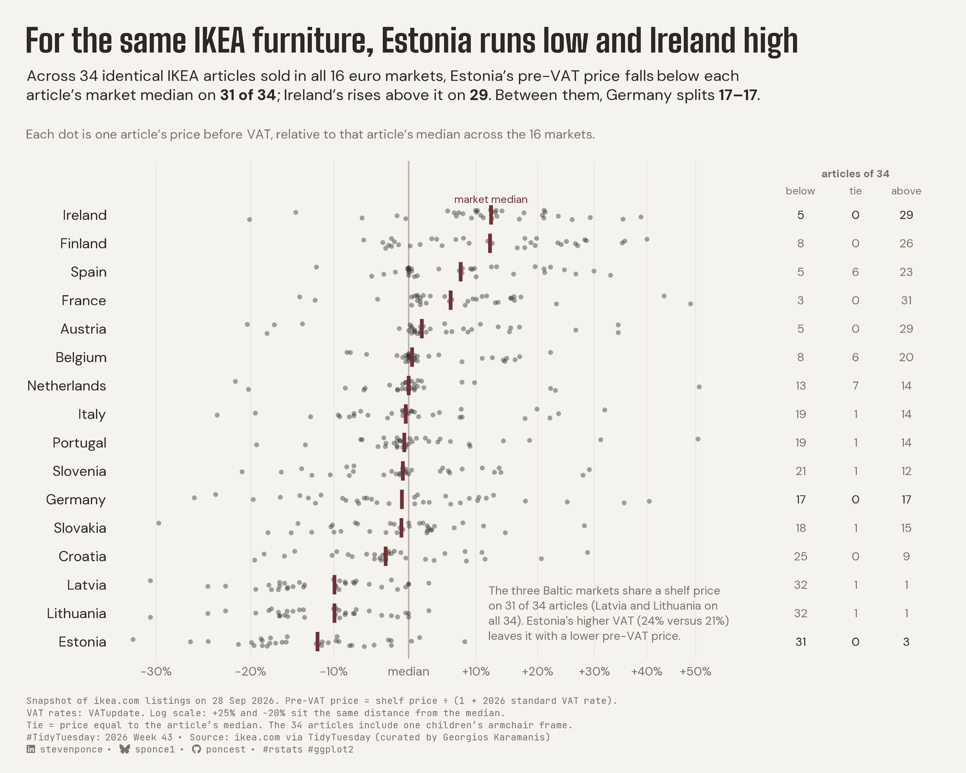
Across 34 identical IKEA articles sold in all 16 euro markets, Estonia’s pre-VAT price falls below each article’s market median on 31 of 34; Ireland’s rises above it on 29. Between them, Germany splits 17–17.

A dot plot comparing the pre-VAT prices of 34 identical IKEA articles across all 16 euro markets shows Estonia consistently low and Ireland consistently high, while mid-table markets like Germany split evenly. Prices are VAT-adjusted and indexed to each article’s own median, removing currency and tax effects. Built in R with ggplot2, ggtext and showtext.

Figure 1: Strip plot titled “For the same IKEA furniture, Estonia runs low and Ireland high.” Sixteen euro markets are stacked as rows, and each row has 34 grey dots, one per identical IKEA article, placed by its pre-VAT price relative to that article’s median across the 16 markets, on a log scale from minus 30 to plus 50 percent. A burgundy tick marks each market’s median. Estonia sits lowest: below the article median on 31 of 34 articles, with a median about 12 percent under. Ireland and Finland sit highest, about 12 percent over; Ireland is above on 29 of 34. Mid-table markets such as Germany split 17 below and 17 above. A right-hand column lists below, tie, and above counts for every market. A note explains that the three Baltic markets share a shelf price on 31 of 34 articles, so Estonia’s higher VAT leaves it with a lower pre-VAT price. Data: IKEA.com listings on 28 September 2026, via TidyTuesday.

Steps to Create this Graphic

1. Load Packages & Setup

```{r}
#| label: load
#| warning: false
#| message: false      
#| results: "hide"     

## 1. LOAD PACKAGES & SETUP ----
suppressPackageStartupMessages({
if (!require("pacman")) install.packages("pacman")
pacman::p_load(
    tidyverse, ggtext, showtext, janitor, scales, 
    glue, ggview, magick
    )
})

# Source utility functions
suppressMessages(source(here::here("R/utils/fonts.R")))
source(here::here("R/utils/social_icons.R"))
source(here::here("R/utils/image_utils.R"))
source(here::here("R/themes/base_theme.R"))
```

2. Read in the Data

```{r}
#| label: read
#| include: true
#| eval: true
#| warning: false

### |- figure settings ----
fig_w   <- 10
fig_h   <- 8
fig_dpi <- 320
out_file   <- "2026/Week_43/2026_43.png"

setup_fonts()
fonts <- get_font_families()


## 2. READ IN THE DATA ----
tt <- tidytuesdayR::tt_load(2026, week = 43)
ikea_seating_raw <- tt$ikea_seating |> clean_names()
rm(tt)
```

3. Examine the Data

```{r}
#| label: examine
#| include: true
#| eval: true
#| results: 'hide'
#| warning: false

## 3. EXAMINING THE DATA ----
glimpse(ikea_seating_raw)
skimr::skim(ikea_seating_raw)
```

4. Tidy Data

```{r}
#| label: tidy
#| warning: false

### |- 2026 standard VAT rates, euro markets ----
vat_rates <- c(
  at = 0.20, be = 0.21, de = 0.19, ee = 0.24, es = 0.21, fi = 0.255,
  fr = 0.20, hr = 0.25, ie = 0.23, it = 0.22, lt = 0.21, lv = 0.21,
  nl = 0.21, pt = 0.23, si = 0.22, sk = 0.23
)

market_names <- c(
  at = "Austria", be = "Belgium", de = "Germany", ee = "Estonia",
  es = "Spain", fi = "Finland", fr = "France", hr = "Croatia",
  ie = "Ireland", it = "Italy", lt = "Lithuania", lv = "Latvia",
  nl = "Netherlands", pt = "Portugal", si = "Slovenia", sk = "Slovakia"
)

### |- euro listings, one row per market x article ----
euro <- ikea_seating_raw |>
  filter(currency == "EUR") |>
  distinct(country, item_no, .keep_all = TRUE) |>
  mutate(price_net = price / (1 + unname(vat_rates[country])))


### |- fixed cohort: articles listed in all 16 euro markets ----
cohort <- euro |>
  add_count(item_no, name = "n_markets") |>
  filter(n_markets == 16) |>
  mutate(
    article_median = median(price_net),
    rel_price = price_net / article_median,
    side = case_when(
      price_net < article_median - 0.005 ~ "below",
      price_net > article_median + 0.005 ~ "above",
      TRUE ~ "tie"
    ),
    .by = item_no
  )

### |- per-market summary ----
market_summary <- cohort |>
  summarise(
    median_rel = median(rel_price),
    below = sum(side == "below"),
    tie = sum(side == "tie"),
    above = sum(side == "above"),
    .by = country
  ) |>
  mutate(market = unname(market_names[country])) |>
  arrange(median_rel)

market_levels <- market_summary$market # cheapest at the bottom

cohort <- cohort |>
  mutate(market = factor(unname(market_names[country]), levels = market_levels))

market_summary <- market_summary |>
  mutate(
    market = factor(market, levels = market_levels),
    named = country %in% c("ee", "ie", "de")
  )

### |- counts quoted in the copy ----
n_ee_below <- market_summary$below[market_summary$country == "ee"]
n_ie_above <- market_summary$above[market_summary$country == "ie"]
n_de_below <- market_summary$below[market_summary$country == "de"]
n_de_above <- market_summary$above[market_summary$country == "de"]

# Baltic markets: shared shelf price (with VAT), different VAT
baltic_prices <- cohort |>
  filter(country %in% c("ee", "lv", "lt")) |>
  select(item_no, country, price) |>
  pivot_wider(names_from = country, values_from = price)

n_baltic_same <- sum(baltic_prices$ee == baltic_prices$lv & baltic_prices$lv == baltic_prices$lt)
n_lv_lt_same <- sum(baltic_prices$lv == baltic_prices$lt)

### |- count-column layout (secondary to the dots) ----
count_cols <- tibble(
  side = c("below", "tie", "above"),
  x = c(1.74, 1.88, 2.02)
)

count_labels <- market_summary |>
  select(market, named, below, tie, above) |>
  pivot_longer(c(below, tie, above), names_to = "side", values_to = "n") |>
  left_join(count_cols, by = "side")
```

5. Visualization Parameters

```{r}
#| label: params
#| include: true
#| warning: false

### |- plot aesthetics ----
clrs <- get_theme_colors(
  palette = list(
    dot = "#2C2825",
    median = "#722F37",
    ref = "#B9B1A6",
    muted = "#7A7068",
    ink = "#2C2825"
  )
)

### |- titles and caption ----
title_text <- "For the same IKEA furniture, Estonia runs low and Ireland high"

subtitle_text <- str_glue(
  "Across 34 identical IKEA articles sold in all 16 euro markets, Estonia's pre-VAT price falls below each<br>",
  "article's market median on **{n_ee_below} of 34**; Ireland's rises above it on **{n_ie_above}**. ",
  "Between them, Germany splits **{n_de_below}–{n_de_above}**.<br><br>",
  "<span style='font-size:9.5pt;color:#7A7068'>Each dot is one article's price before VAT, relative to that article's ",
  "median across the 16 markets.</span>"
)

annotation_text <- str_glue(
  "The three Baltic markets share a shelf price on {n_baltic_same} of 34 articles ",
  "(Latvia and Lithuania on all {n_lv_lt_same}). Estonia's higher VAT (24% versus 21%) ",
  "leaves it with a lower pre-VAT price."
)

disclosure_text <- paste0(
  "Snapshot of ikea.com listings on 28 Sep 2026. Pre-VAT price = shelf price ÷ (1 + 2026 standard VAT rate).<br>",
  "VAT rates: VATupdate. Log scale: +25% and −20% sit the same distance from the median.<br>",
  "Tie = price equal to the article's median. The 34 articles include one children's armchair frame."
)

caption_text <- paste0(
  disclosure_text, "<br>",
  create_social_caption(
    tt_year = 2026,
    tt_week = 43,
    source_text = "ikea.com via TidyTuesday (curated by Georgios Karamanis)"
  )
)

### |- plot theme ----
base_theme <- create_base_theme(clrs)

weekly_theme <- extend_weekly_theme(
  base_theme,
  theme(
    plot.title = element_text(
      face = "bold", family = fonts$title_1, size = 24,
      color = "#2C2825", margin = margin(b = 8)
    ),
    plot.subtitle = element_markdown(
      family = fonts$subtitle, size = 11.5, color = "#2C2825",
      lineheight = 1.25, margin = margin(b = 14)
    ),
    plot.caption = element_markdown(
      family = fonts$caption, size = 7, color = "#7A7068",
      hjust = 0, lineheight = 1.3, margin = margin(t = 14)
    ),
    plot.title.position = "plot",
    plot.caption.position = "plot",
    axis.text.y = element_text(family = fonts$text, size = 10.5, color = "#2C2825", hjust = 1),
    axis.text.x = element_text(family = fonts$text, size = 9, color = "#7A7068"),
    axis.title = element_blank(),
    axis.ticks = element_blank(),
    panel.grid.major.x = element_line(color = "gray90", linewidth = 0.3),
    panel.grid.major.y = element_blank(),
    panel.grid.minor = element_blank(),
    legend.position = "none",
    plot.margin = margin(20, 24, 14, 20)
  )
)

theme_set(weekly_theme)
```

6. Plot

```{r}
#| label: plot
#| warning: false

### |-  main plot ----

### |- axis: percent from the article median, on a log scale ----
x_breaks <- c(0.7, 0.8, 0.9, 1, 1.1, 1.2, 1.3, 1.4, 1.5)
x_labels <- c("−30%", "−20%", "−10%", "median", "+10%", "+20%", "+30%", "+40%", "+50%")

p <- ggplot(cohort, aes(x = rel_price, y = market)) +

  # reference line at the article median
  geom_vline(xintercept = 1, color = "#B9B1A6", linewidth = 0.5) +

  # one dot per article
  geom_point(
    position = position_jitter(height = 0.18, width = 0, seed = 43),
    color = "#2C2825", alpha = 0.42, size = 1.7, stroke = 0
  ) +

  # market median tick
  geom_segment(
    data = market_summary,
    aes(
      x = median_rel, xend = median_rel,
      y = as.integer(market) - 0.34, yend = as.integer(market) + 0.34
    ),
    color = "#722F37", linewidth = 1.3, lineend = "butt"
  ) +

  # direct label for the median tick, on the top row only
  annotate(
    "text",
    x = market_summary$median_rel[market_summary$market == last(market_levels)],
    y = length(market_levels) + 0.55,
    label = "market median",
    family = fonts$text, size = 2.8, color = "#722F37", hjust = 0.5
  ) +

  # count column, secondary: grey, small, named markets in ink
  geom_text(
    data = count_labels,
    aes(x = x, y = market, label = n, color = named),
    family = fonts$text, size = 3.1, hjust = 0.5
  ) +
  annotate(
    "text",
    x = count_cols$x, y = length(market_levels) + 0.85,
    label = count_cols$side,
    family = fonts$text, size = 2.8, color = "#7A7068", hjust = 0.5
  ) +
  annotate(
    "text",
    x = mean(count_cols$x), y = length(market_levels) + 1.45,
    label = "articles of 34",
    family = fonts$text, size = 2.8, color = "#7A7068", fontface = "bold", hjust = 0.5
  ) +

  # Estonia-Latvia annotation, in the empty right side of the Baltic rows
  annotate(
    "text",
    x = 1.12, y = 2,
    label = str_wrap(annotation_text, 46), # 46 keeps "24% versus 21%" on one line, no orphan
    family = fonts$text, size = 3, color = "#7A7068",
    hjust = 0, vjust = 0.5, lineheight = 1.1
  ) +
  scale_color_manual(values = c(`TRUE` = "#2C2825", `FALSE` = "#7A7068"), guide = "none") +
  scale_x_log10(
    breaks = x_breaks, labels = x_labels,
    limits = c(0.66, 2.1), expand = expansion(0)
  ) +
  scale_y_discrete(expand = expansion(add = c(0.6, 1.9))) +
  labs(
    title = title_text,
    subtitle = subtitle_text,
    caption = caption_text
  )
```

7. Save

```{r}
#| label: save
#| warning: false

### |- save ----
main_path  <- here::here("data_visualizations", "TidyTuesday", "2026", "tt_2026_43.png")
thumb_path <- here::here("data_visualizations", "TidyTuesday", "2026", "thumbnails", "tt_2026_43.png")

# Full-size version, for the QMD figure
ggview::save_ggplot(plot = p, file   = main_path, width  = fig_w,
    height = fig_h, units  = "in", dpi = fig_dpi)

# Reduced-size thumbnail, for the YAML `image:` field
fs::dir_create(dirname(thumb_path))
magick::image_read(main_path) |>
  magick::image_resize("400") |>
  magick::image_write(thumb_path)
```

8. Session Info

TipExpand for Session Info

R version 4.6.1 (2026-06-24)
Platform: aarch64-apple-darwin23
Running under: macOS Tahoe 26.6.2

Matrix products: default
BLAS:   /Library/Frameworks/R.framework/Versions/4.6/Resources/lib/libRblas.0.dylib 
LAPACK: /Library/Frameworks/R.framework/Versions/4.6/Resources/lib/libRlapack.dylib;  LAPACK version 3.12.1

locale:
[1] en_US.UTF-8/en_US.UTF-8/en_US.UTF-8/C/en_US.UTF-8/en_US.UTF-8

time zone: America/New_York
tzcode source: internal

attached base packages:
[1] stats     graphics  grDevices utils     datasets  methods   base     

other attached packages:
 [1] here_1.0.2      magick_2.9.1    ggview_0.2.2    glue_1.8.1     
 [5] scales_1.4.0    janitor_2.2.1   showtext_0.9-8  showtextdb_3.0 
 [9] sysfonts_0.8.9  ggtext_0.2.0    lubridate_1.9.5 forcats_1.0.1  
[13] stringr_1.6.0   dplyr_1.2.1     purrr_1.2.2     readr_2.2.0    
[17] tidyr_1.3.2     tibble_3.3.1    ggplot2_4.0.3   tidyverse_2.0.0
[21] pacman_0.5.1   

loaded via a namespace (and not attached):
 [1] gtable_0.3.6       xfun_0.60          httr2_1.3.0        htmlwidgets_1.6.4 
 [5] gh_1.6.1           tzdb_0.5.0         vctrs_0.7.3        tools_4.6.1       
 [9] generics_0.1.4     curl_7.1.0         parallel_4.6.1     pkgconfig_2.0.3   
[13] RColorBrewer_1.1-3 skimr_2.2.2        S7_0.2.2           lifecycle_1.0.5   
[17] compiler_4.6.1     farver_2.1.2       textshaping_1.0.5  repr_1.1.7        
[21] codetools_0.2-20   snakecase_0.11.1   litedown_0.10      htmltools_0.5.9   
[25] yaml_2.3.12        pillar_1.11.1      crayon_1.5.3       commonmark_2.0.0  
[29] tidyselect_1.2.1   digest_0.6.39      stringi_1.8.7      rprojroot_2.1.1   
[33] fastmap_1.2.0      grid_4.6.1         cli_3.6.6          magrittr_2.0.5    
[37] base64enc_0.1-6    withr_3.0.3        bit64_4.8.2        timechange_0.4.0  
[41] rmarkdown_2.31     tidytuesdayR_1.3.2 gitcreds_0.1.2     bit_4.6.0         
[45] otel_0.2.0         ragg_1.5.2         hms_1.1.4          evaluate_1.0.5    
[49] knitr_1.51         markdown_2.0       rlang_1.3.0        gridtext_0.1.6    
[53] Rcpp_1.1.2         xml2_1.6.0         rstudioapi_0.19.0  vroom_1.7.1       
[57] jsonlite_2.0.0     R6_2.6.1           fs_2.1.0           systemfonts_1.3.2 

9. GitHub Repository

TipExpand for GitHub Repo

The complete code for this analysis is available in tt_2026_43.qmd.

For the full repository, click here.

10. References

TipExpand for References

1. Data Source:
   • TidyTuesday 2026 Week 43: IKEA Sofas and Their Swedish Places

11. Custom Functions Documentation

Note📦 Custom Helper Functions

This analysis uses custom functions from my personal module library for efficiency and consistency across projects.

Functions Used:

• fonts.R: setup_fonts(), get_font_families() - Font management with showtext
• social_icons.R: create_social_caption() - Generates formatted social media captions
• image_utils.R: save_plot() - Consistent plot saving with naming conventions
• base_theme.R: create_base_theme(), extend_weekly_theme(), get_theme_colors() - Custom ggplot2 themes

Why custom functions?
These utilities standardize theming, fonts, and output across all my data visualizations. The core analysis (data tidying and visualization logic) uses only standard tidyverse packages.

Source Code:
View all custom functions → GitHub: R/utils