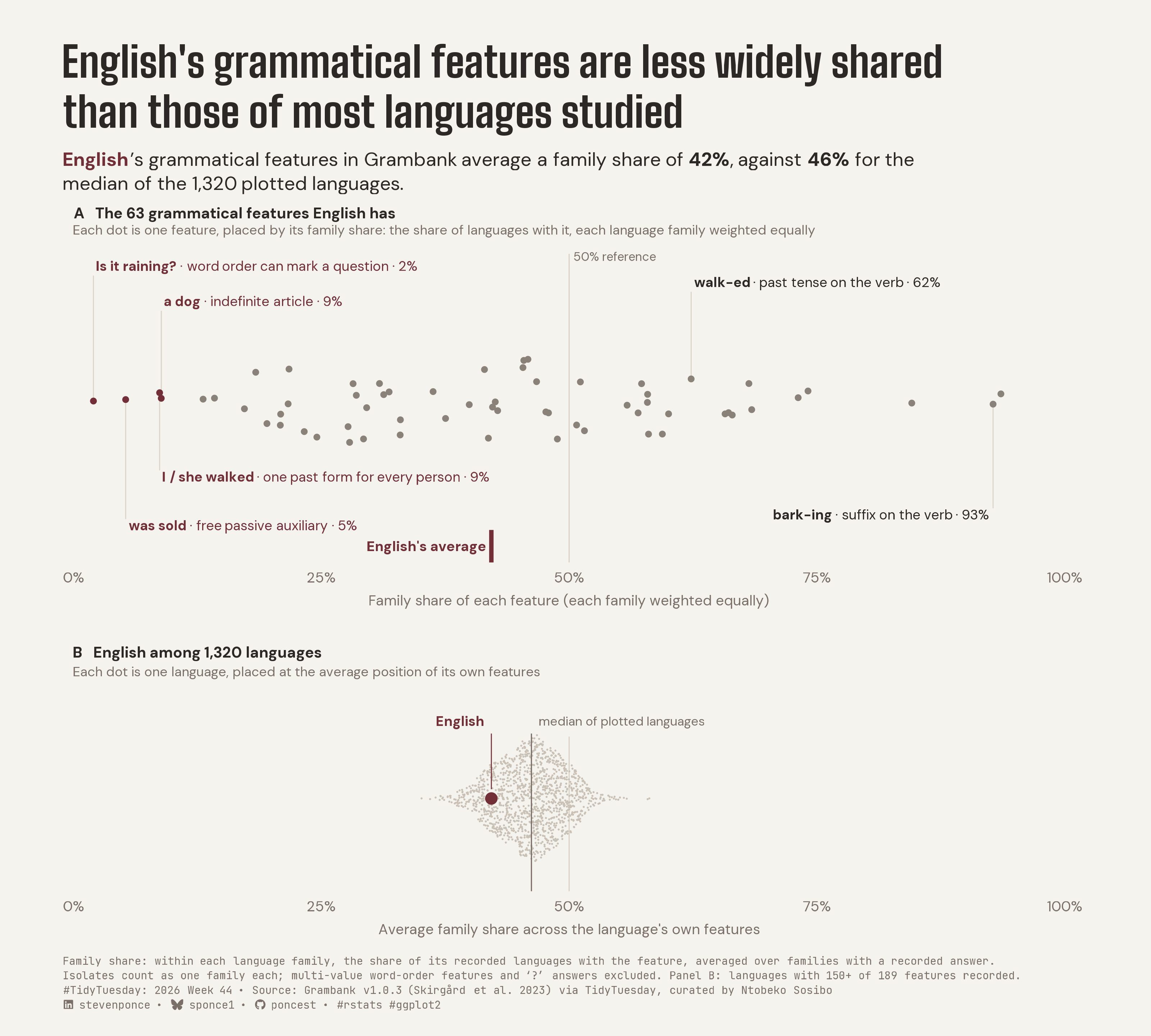
English’s grammatical features are less widely shared than those of most languages studied

English’s grammatical features in Grambank average a family share of 42%, against 46% for the median of the 1,320 plotted languages.

English’s 63 recorded grammatical features average a family share of 42%, below the 46% median of 1,320 languages in Grambank. Each feature is weighted so every language family counts equally, and each language is placed at the average of its own features on a shared scale. Built in R with ggplot2, ggbeeswarm, patchwork and ggtext.

Figure 1: Two-panel beeswarm chart titled “English’s grammatical features are less widely shared than those of most languages studied.” English’s features average a family share of 42% (the share of languages with a feature, each language family weighted equally), against 46% for the median of 1,320 plotted languages. Panel A places English’s 63 grammatical features on a 0–100% family-share axis, with a burgundy tick marking English’s average. Four rare features are highlighted in burgundy: word order can mark a question (“Is it raining?”, 2%), a free passive auxiliary (“was sold”, 5%), an indefinite article (“a dog”, 9%), and one past form for every person (“I/she walked”, 9%). Two common controls appear for contrast: past tense on the verb (62%) and a verb suffix (93%). Panel B plots each language at the average family share of its own features; they form a narrow cloud between about 35% and 58%, with English on the left. Source: Grambank v1.0.3 via TidyTuesday.

Steps to Create this Graphic

1. Load Packages & Setup

```{r}
#| label: load
#| warning: false
#| message: false      
#| results: "hide"     

## 1. LOAD PACKAGES & SETUP ----
suppressPackageStartupMessages({
if (!require("pacman")) install.packages("pacman")
pacman::p_load(
    tidyverse, ggtext, showtext, scales, glue, ggview,
    ggbeeswarm, patchwork, ragg
    )
})

# Source utility functions
suppressMessages(source(here::here("R/utils/fonts.R")))
source(here::here("R/utils/social_icons.R"))
source(here::here("R/utils/image_utils.R"))
source(here::here("R/themes/base_theme.R"))
```

2. Read in the Data

```{r}
#| label: read
#| include: true
#| eval: true
#| warning: false

### |- figure settings ----
fig_w   <- 10
fig_h   <- 9
fig_dpi <- 320

### |- fonts ----
setup_fonts()
fonts <- get_font_families()
title_family <- fonts$title_1


## 2. READ IN THE DATA ----
## Read every field as character with no NA tokens: Grambank writes isolates' family as
## the literal "NA", and tt_load() cannot be told otherwise.
tt_url <- "https://raw.githubusercontent.com/rfordatascience/tidytuesday/main/data/2026/2026-11-03/"
read_chr <- function(url) {
  read_csv(url, col_types = cols(.default = col_character()), na = character(), show_col_types = FALSE)
}

languages_raw <- read_chr(paste0(tt_url, "grambank_languages.csv"))
parameters_raw <- read_chr(paste0(tt_url, "grambank_parameters.csv"))
values_raw <- read_chr(paste0(tt_url, "grambank_values.csv"))

# Grambank's own languages table (v1.0.3, same release as the TT extract): variety level and
# language-level ID, which the TT extract drops
gb_languages_raw <- read_chr("https://raw.githubusercontent.com/grambank/grambank/v1.0.3/cldf/languages.csv")
```

3. Examine the Data

```{r}
#| label: examine
#| include: true
#| eval: true
#| results: 'hide'
#| warning: false

## 3. EXAMINING THE DATA ----
glimpse(languages_raw)
glimpse(parameters_raw)
glimpse(values_raw)
```

4. Tidy Data

```{r}
#| label: tidy
#| warning: false

### |- analysis frame: one variety per language, no proto-languages ----
multistate_ids <- c("GB024", "GB025", "GB065", "GB130", "GB193", "GB203")

coded_counts <- values_raw |> count(language_id, name = "n_coded")

analysis_ids <- gb_languages_raw |>
  filter(level != "family") |>
  left_join(coded_counts, by = c("ID" = "language_id")) |>
  slice_max(n_coded, n = 1, with_ties = FALSE, by = Language_level_ID) |>
  pull(ID)

languages <- languages_raw |>
  filter(language_id %in% analysis_ids) |>
  mutate(family_unit = if_else(family_name == "NA", paste0("isolate_", language_id), family_name))

binary_values <- values_raw |>
  filter(!parameter_id %in% multistate_ids, language_id %in% analysis_ids) |>
  mutate(present = as.integer(value)) |>
  left_join(languages |> select(language_id, family_unit), by = "language_id")

### |- family-balanced share for each feature ----
## within each family: share of its recorded languages with the feature;
## then the mean over families with a recorded answer (each isolate is one family)
feature_share <- binary_values |>
  summarise(family_rate = mean(present), .by = c(parameter_id, family_unit)) |>
  summarise(family_share = mean(family_rate), n_families = n(), .by = parameter_id)

### |- English's present features (panel A) ----
english_id <- "stan1293"
english_features <- binary_values |>
  filter(language_id == english_id, present == 1) |>
  left_join(feature_share, by = "parameter_id")

### |- each language's average (panel B) ----
min_recorded <- 150
language_avg <- binary_values |>
  left_join(feature_share, by = "parameter_id") |>
  summarise(n_recorded = n(), avg_share = mean(family_share[present == 1]), .by = language_id) |>
  filter(n_recorded >= min_recorded)

english_avg <- language_avg$avg_share[language_avg$language_id == english_id]
median_avg <- median(language_avg$avg_share)
share_more_common <- mean(language_avg$avg_share > english_avg)

### |- named features: four rarest English features + two widely shared controls ----
named_features <- tribble(
  ~parameter_id, ~example,          ~device,                          ~side,
  "GB260",       "Is it raining?",  "word order can mark a question", "rare",
  "GB302",       "was sold",        "free passive auxiliary",         "rare",
  "GB021",       "a dog",           "indefinite article",             "rare",
  "GB400",       "I / she walked",  "one past form for every person", "rare",
  "GB083",       "walk-ed",         "past tense on the verb",         "control",
  "GB080",       "bark-ing",        "suffix on the verb",             "control"
)
```

5. Visualization Parameters

```{r}
#| label: params
#| include: true
#| warning: false

### |- plot aesthetics ----
clrs <- get_theme_colors(
  palette = list(
    accent = "#722F37",
    ink    = "#2C2825",
    dot    = "#8A8178",
    cloud  = "#C9C1B6",
    ref    = "#D9D3C9",
    muted  = "#7A7068"
  )
)
col_accent <- clrs$palette$accent
col_ink <- clrs$palette$ink
col_dot <- clrs$palette$dot
col_cloud <- clrs$palette$cloud
col_ref <- clrs$palette$ref
col_muted <- clrs$palette$muted

### |- titles and caption ----
title_text <- "English's grammatical features are less widely shared\nthan those of most languages studied"

subtitle_text <- glue(
  "<span style='color:{col_accent}'>**English**</span>'s grammatical features in Grambank average a family share of ",
  "**{round(100 * english_avg)}%**, against **{round(100 * median_avg)}%** for the<br>median of the {comma(nrow(language_avg))} plotted languages."
)

cue_a <- "Each dot is one feature, placed by its family share: the share of languages with it, each language family weighted equally"

caption_lines <- c(
  "Family share: within each language family, the share of its recorded languages with the feature, averaged over families with a recorded answer.",
  glue(
    "Isolates count as one family each; multi-value word-order features and '?' answers excluded. ",
    "Panel B: languages with {min_recorded}+ of 189 features recorded."
  )
)

disclosure_text <- glue(
  "{caption_lines[1]}<br>{caption_lines[2]}"
)

caption_text <- paste0(
  disclosure_text, "<br>",
  create_social_caption(
    tt_year = 2026,
    tt_week = 44,
    source_text = "Grambank v1.0.3 (Skirgård et al. 2023) via TidyTuesday, curated by Ntobeko Sosibo"
  )
)

### |- plot theme ----
base_theme <- create_base_theme(clrs)

weekly_theme <- extend_weekly_theme(
  base_theme,
  theme(
    plot.title = element_text(
      face = "bold", family = title_family, size = 26,
      color = col_ink, lineheight = 1.0, margin = margin(b = 10)
    ),
    plot.subtitle = element_markdown(
      family = fonts$subtitle, size = 12, color = col_ink,
      lineheight = 1.25, margin = margin(b = 6)
    ),
    plot.caption = element_markdown(
      family = fonts$caption, size = 6.8, color = col_muted,
      hjust = 0, lineheight = 1.35, margin = margin(t = 12)
    ),
    axis.text.x = element_text(family = fonts$text, size = 9, color = col_muted),
    axis.title.x = element_text(
      family = fonts$text, size = 9, color = col_muted,
      face = "plain", margin = margin(t = 6)
    ),
    axis.text.y = element_blank(),
    axis.title.y = element_blank(),
    axis.ticks = element_blank(),
    panel.grid = element_blank(),
    legend.position = "none",
    plot.margin = margin(14, 24, 8, 20)
  )
)

theme_set(weekly_theme)

### |- shared x scale ----
x_scale <- scale_x_continuous(
  limits = c(0, 1), breaks = seq(0, 1, 0.25),
  labels = label_percent(), expand = expansion(add = c(0.01, 0.01))
)
```

6. Plot

```{r}
#| label: plot
#| warning: false

### |- panel A: English's 63 features ----
set.seed(2026)
swarm_a <- layer_data(
  ggplot(english_features, aes(family_share, 0)) +
    geom_quasirandom(orientation = "y", width = 0.32, method = "pseudorandom", )
) |>
  select(x, y) |>
  bind_cols(english_features |> select(parameter_id, family_share))

labels_a <- named_features |>
  left_join(swarm_a, by = "parameter_id") |>
  mutate(
    pct = round(100 * family_share),
    label = glue("<b>{example}</b> · {device} · {pct}%"),
    label_y = c(0.92, -0.88, 0.66, -0.52, 0.80, -0.80),
    hjust = case_when(parameter_id == "GB080" ~ 1, TRUE ~ 0),
    colour = if_else(side == "rare", col_accent, col_ink)
  )

p_a <- ggplot(swarm_a, aes(x, y)) +
  annotate("segment", x = 0.5, xend = 0.5, y = -1.2, yend = 1.08, color = col_ref, linewidth = 0.35) +
  annotate("text",
    x = 0.505, y = 1.06, label = "50% reference",
    family = fonts$text, size = 2.7, color = col_muted, hjust = 0
  ) +
  geom_segment(
    data = labels_a, aes(x = x, xend = x, y = y, yend = label_y),
    color = col_ref, linewidth = 0.3
  ) +
  geom_point(aes(color = family_share < 0.10), size = 2, stroke = 0) +
  geom_richtext(
    data = labels_a,
    aes(x = x, y = label_y, label = label, hjust = hjust),
    color = labels_a$colour, family = fonts$text, size = 3, fill = NA, label.colour = NA,
    label.padding = unit(c(1, 2, 1, 2), "pt"), vjust = if_else(labels_a$label_y > 0, 0, 1)
  ) +
  annotate("segment",
    x = english_avg, xend = english_avg, y = -1.20, yend = -0.96,
    color = col_accent, linewidth = 1.3, lineend = "butt"
  ) +
  annotate("text",
    x = english_avg - 0.006, y = -1.08, label = "English's average",
    family = fonts$text, size = 3.1, color = col_accent, fontface = "bold", hjust = 1
  ) +
  annotate("text",
    x = 0, y = 1.42, hjust = 0, vjust = 1, family = fonts$text, size = 3.3,
    color = col_ink, fontface = "bold", label = "A   The 63 grammatical features English has"
  ) +
  annotate("text",
    x = 0, y = 1.29, hjust = 0, vjust = 1, family = fonts$text, size = 2.9,
    color = col_muted,
    label = cue_a
  ) +
  scale_color_manual(values = c(`TRUE` = col_accent, `FALSE` = col_dot)) +
  x_scale +
  scale_y_continuous(limits = c(-1.2, 1.45), expand = expansion(0)) +
  labs(
    title = title_text, subtitle = subtitle_text,
    x = "Family share of each feature (each family weighted equally)"
  )

### |- panel B: 1,320 languages at their averages ----
set.seed(2026)
swarm_b <- layer_data(
  ggplot(language_avg, aes(avg_share, 0)) +
    geom_quasirandom(orientation = "y", width = 0.42, method = "pseudorandom")
) |>
  select(x, y)

p_b <- ggplot(language_avg, aes(avg_share, 0)) +
  annotate("segment", x = 0.5, xend = 0.5, y = -0.6, yend = 0.40, color = col_ref, linewidth = 0.35) +
  geom_quasirandom(
    orientation = "y", width = 0.42, method = "pseudorandom",
    size = 0.6, stroke = 0, color = col_cloud
  ) +
  annotate("segment", x = median_avg, xend = median_avg, y = -0.6, yend = 0.42, color = col_muted, linewidth = 0.35) +
  annotate("text",
    x = median_avg + 0.008, y = 0.5, label = "median of plotted languages",
    family = fonts$text, size = 2.8, color = col_muted, hjust = 0
  ) +
  annotate("point", x = english_avg, y = 0, color = col_accent, size = 2.8) +
  annotate("segment",
    x = english_avg, xend = english_avg, y = 0.06, yend = 0.42,
    color = col_accent, linewidth = 0.3
  ) +
  annotate("text",
    x = english_avg - 0.008, y = 0.5, label = "English",
    family = fonts$text, size = 3, color = col_accent, fontface = "bold", hjust = 1
  ) +
  annotate("text",
    x = 0, y = 0.98, hjust = 0, vjust = 1, family = fonts$text, size = 3.3,
    color = col_ink, fontface = "bold",
    label = glue("B   English among {comma(nrow(language_avg))} languages")
  ) +
  annotate("text",
    x = 0, y = 0.85, hjust = 0, vjust = 1, family = fonts$text, size = 2.9,
    color = col_muted,
    label = "Each dot is one language, placed at the average position of its own features"
  ) +
  x_scale +
  scale_y_continuous(limits = c(-0.6, 1.0), expand = expansion(0)) +
  labs(
    x = "Average family share across the language's own features",
    caption = caption_text
  )

### |- combine ----
p <- p_a / p_b + plot_layout(heights = c(1.45, 1))
```

7. Save

```{r}
#| label: save
#| warning: false

### |- save ----
main_path  <- here::here("data_visualizations", "TidyTuesday", "2026", "tt_2026_44.png")
thumb_path <- here::here("data_visualizations", "TidyTuesday", "2026", "thumbnails", "tt_2026_44.png")

# Full-size version, for the QMD figure
ggview::save_ggplot(plot = p, file   = main_path, width  = fig_w,
    height = fig_h, units  = "in", dpi = fig_dpi)

# Reduced-size thumbnail, for the YAML `image:` field
fs::dir_create(dirname(thumb_path))
magick::image_read(main_path) |>
  magick::image_resize("400") |>
  magick::image_write(thumb_path)
```

8. Session Info

TipExpand for Session Info

R version 4.6.1 (2026-06-24)
Platform: aarch64-apple-darwin23
Running under: macOS Tahoe 26.6.2

Matrix products: default
BLAS:   /Library/Frameworks/R.framework/Versions/4.6/Resources/lib/libRblas.0.dylib 
LAPACK: /Library/Frameworks/R.framework/Versions/4.6/Resources/lib/libRlapack.dylib;  LAPACK version 3.12.1

locale:
[1] en_US.UTF-8/en_US.UTF-8/en_US.UTF-8/C/en_US.UTF-8/en_US.UTF-8

time zone: America/New_York
tzcode source: internal

attached base packages:
[1] stats     graphics  grDevices utils     datasets  methods   base     

other attached packages:
 [1] here_1.0.2       ragg_1.5.2       patchwork_1.3.2  ggbeeswarm_0.7.3
 [5] ggview_0.2.2     glue_1.8.1       scales_1.4.0     showtext_0.9-8  
 [9] showtextdb_3.0   sysfonts_0.8.9   ggtext_0.2.0     lubridate_1.9.5 
[13] forcats_1.0.1    stringr_1.6.0    dplyr_1.2.1      purrr_1.2.2     
[17] readr_2.2.0      tidyr_1.3.2      tibble_3.3.1     ggplot2_4.0.3   
[21] tidyverse_2.0.0  pacman_0.5.1    

loaded via a namespace (and not attached):
 [1] gtable_0.3.6       beeswarm_0.4.0     xfun_0.60          htmlwidgets_1.6.4 
 [5] tzdb_0.5.0         vctrs_0.7.3        tools_4.6.1        generics_0.1.4    
 [9] curl_7.1.0         parallel_4.6.1     pkgconfig_2.0.3    RColorBrewer_1.1-3
[13] S7_0.2.2           lifecycle_1.0.5    compiler_4.6.1     farver_2.1.2      
[17] textshaping_1.0.5  codetools_0.2-20   litedown_0.10      vipor_0.4.7       
[21] htmltools_0.5.9    yaml_2.3.12        pillar_1.11.1      crayon_1.5.3      
[25] magick_2.9.1       commonmark_2.0.0   tidyselect_1.2.1   digest_0.6.39     
[29] stringi_1.8.7      labeling_0.4.3     rprojroot_2.1.1    fastmap_1.2.0     
[33] grid_4.6.1         cli_3.6.6          magrittr_2.0.5     withr_3.0.3       
[37] bit64_4.8.2        timechange_0.4.0   rmarkdown_2.31     bit_4.6.0         
[41] otel_0.2.0         hms_1.1.4          evaluate_1.0.5     knitr_1.51        
[45] markdown_2.0       rlang_1.3.0        gridtext_0.1.6     Rcpp_1.1.2        
[49] xml2_1.6.0         rstudioapi_0.19.0  vroom_1.7.1        jsonlite_2.0.0    
[53] R6_2.6.1           fs_2.1.0           systemfonts_1.3.2 

9. GitHub Repository

TipExpand for GitHub Repo

The complete code for this analysis is available in tt_2026_44.qmd.

For the full repository, click here.

10. References

TipExpand for References

1. Data Source:
   • TidyTuesday 2026 Week 44: Grambank

11. Custom Functions Documentation

Note📦 Custom Helper Functions

This analysis uses custom functions from my personal module library for efficiency and consistency across projects.

Functions Used:

• fonts.R: setup_fonts(), get_font_families() - Font management with showtext
• social_icons.R: create_social_caption() - Generates formatted social media captions
• base_theme.R: create_base_theme(), extend_weekly_theme(), get_theme_colors() - Custom ggplot2 themes

Why custom functions?
These utilities standardize theming, fonts, and output across all my data visualizations. The core analysis (data tidying and visualization logic) uses only standard tidyverse packages.

Source Code:
View all custom functions → GitHub: R/utils