Steven Ponce home pageSteven Ponce home page Steven Ponce
  • About
  • Data Visualizations
  • Projects
  • Behind the Viz
  • Resume
  • Email

On this page

  • Steps to Create this Graphic
    • 1. Load Packages & Setup
    • 2. Read in the Data
    • 3. Examine the Data
    • 4. Tidy Data
    • 5. Visualization Parameters
    • 6. Plot
    • 7. Save
    • 8. Session Info
    • 9. GitHub Repository
    • 10. References
    • 11. Custom Functions Documentation

Cholesterol’s link to death looks different at different ages

  • Show All Code
  • Hide All Code

  • View Source

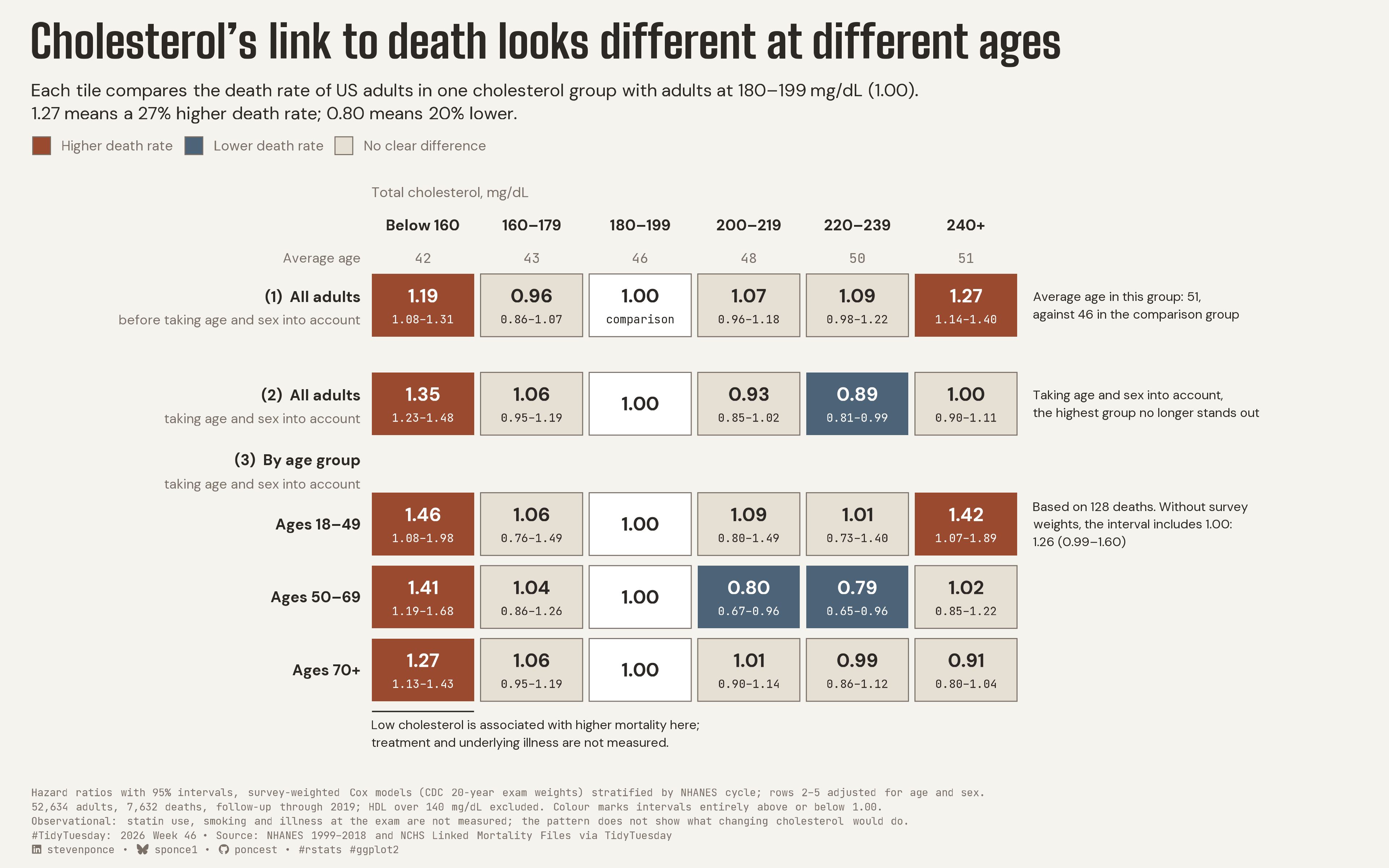
Each tile compares the death rate of US adults in one cholesterol group with adults at 180–199 mg/dL (1.00). 1.27 means a 27% higher death rate; 0.80 means 20% lower.

TidyTuesday
2026
US adults with total cholesterol of 240+ mg/dL had a 27% higher death rate than those at 180–199, but that excess was no longer detectable after taking age and sex into account, and the pattern differed by age group. Survey-weighted Cox models on NHANES 1999–2018 linked to mortality through 2019. Built in R with ggplot2, ggtext, survival and survey.
Author

Steven Ponce

Published

November 16, 2026

Figure 1: Tile matrix titled Cholesterol’s link to death looks different at different ages. Each tile compares the death rate of US adults in one total cholesterol group with adults at 180 to 199 mg/dL, set at 1.00. Before taking age and sex into account, adults at 240+ mg/dL had a 27% higher death rate (1.27); after, the estimate was 1.00, showing no clear difference. Within age groups, the 240+ estimate was 1.42 for ages 18 to 49 (based on 128 deaths and sensitive to survey weighting), 1.02 for ages 50 to 69, and 0.91 for ages 70 and over. Below 160 mg/dL, death rates were higher in every row, from 1.19 to 1.46; treatment and underlying illness were not measured. Average age rose from 42 in the lowest cholesterol group to 51 in the highest. Data: NHANES 1999 to 2018 linked to NCHS mortality records through 2019.

Key takeaways

  • Age matters when comparing cholesterol groups. Adults at 240+ mg/dL averaged 51 years old, versus 46 in the comparison group, and the apparent excess mortality hazard was no longer detectable after adjusting for age and sex.
  • In survey-weighted Cox models of 52,634 adults and 7,632 deaths, the hazard ratio at 240+ mg/dL changed from 1.27 (95% CI 1.14–1.40) to 1.00 (0.90–1.11). The association also differed across age groups (interaction p = 0.00025).
  • Cholesterol below 160 mg/dL was associated with higher mortality hazard in all three age groups, but underlying illness and cholesterol-lowering treatment could contribute to this pattern. The dataset lacks statin use, smoking and baseline illness; the 18–49 high-cholesterol estimate is sensitive to survey weighting. Individual comparisons were not adjusted for multiple testing.

Steps to Create this Graphic

1. Load Packages & Setup

Show code
```{r}
#| label: load
#| warning: false
#| message: false      
#| results: "hide"     

## 1. LOAD PACKAGES & SETUP ----
suppressPackageStartupMessages({
if (!require("pacman")) install.packages("pacman")
pacman::p_load(
    tidyverse, ggtext, showtext, scales, glue, ggview,
    ragg, magick
    )
})

# Source utility functions
suppressMessages(source(here::here("R/utils/fonts.R")))
source(here::here("R/utils/social_icons.R"))
source(here::here("R/utils/image_utils.R"))
source(here::here("R/themes/base_theme.R"))
```

2. Read in the Data

Show code
```{r}
#| label: read
#| include: true
#| eval: true
#| warning: false

### |- figure settings ----
fig_w    <- 12
fig_h    <- 7.5
fig_dpi  <- 320
out_file <- "2026/Week_46/2026_46.png"

### |- fonts ----
setup_fonts()
fonts <- get_font_families()
title_family <- fonts$title_1
title_size   <- 28


## 2. READ IN THE DATA ----
## Read every field as character with no NA tokens; restore numbers column by column.
read_chr <- function(path) {
  read_csv(path, col_types = cols(.default = col_character()), na = character(), show_col_types = FALSE)
}

tt_url <- "https://raw.githubusercontent.com/rfordatascience/tidytuesday/main/data/2026/2026-11-17/"
cm_raw <- read_chr(paste0(tt_url, "cholesterol_mortality.csv"))
est_raw <- read_chr(here::here("data/TidyTuesday/2026/tt_2026_46_estimates.csv"))
```

3. Examine the Data

Show code
```{r}
#| label: examine
#| include: true
#| eval: true
#| results: 'hide'
#| warning: false

## 3. EXAMINING THE DATA ----
glimpse(est_raw)
est_raw |> count(kind, row_key) |> print(n = Inf)
```

4. Tidy Data

Show code
```{r}
#| label: tidy
#| warning: false

### |- analysis population ----
cm <- cm_raw |>
  mutate(across(c(total_chol, hdl, died), \(x) suppressWarnings(as.numeric(na_if(x, "NA")))))
an <- cm |> filter(!is.na(total_chol), !is.na(hdl), hdl <= 140)
n_adults <- nrow(an)
n_deaths <- sum(an$died)

### |- estimates ----
bins_raw <- c("<160", "160-179", "180-199", "200-219", "220-239", "240+")
bins_show <- c("Below 160", "160–179", "180–199", "200–219", "220–239", "240+")

est <- est_raw |>
  mutate(
    across(c(value, lo, hi, deaths), \(x) as.numeric(na_if(x, ""))),
    col = match(bin, bins_raw)
  )

hr <- est |> filter(kind == "hr_weighted")

### |- matrix layout: rows top to bottom = the reading order ----
## groups (1), (2), (3) are separated by wider gaps than rows within a group, so the
## matrix reads as three steps, not one heatmap
row_y <- c(crude_all = 6.3, adj_all = 4.95, adj_18_49 = 3.3, adj_50_69 = 2.3, adj_70p = 1.3)

cells <- hr |>
  mutate(
    y = unname(row_y[row_key]),
    status = case_when(
      bin == "180-199" ~ "ref",
      lo > 1 ~ "higher",
      hi < 1 ~ "lower",
      TRUE ~ "unclear"
    ),
    lab_hr = if_else(status == "ref", "1.00", sprintf("%.2f", value)),
    lab_ci = case_when(
      status == "ref" & row_key == "crude_all" ~ "comparison",
      status == "ref" ~ "",
      TRUE ~ sprintf("%.2f–%.2f", lo, hi)
    ),
    y_hr = if_else(lab_ci == "", y, y + 0.13)
  )

### |- numbers quoted in copy (all from the export) ----
pick <- function(key, b, k = "hr_weighted") est |> filter(kind == k, row_key == key, bin == b)
crude_240 <- pick("crude_all", "240+")
adj_240 <- pick("adj_all", "240+")
young_240 <- pick("adj_18_49", "240+")
young_unw <- pick("adj_18_49", "240+", "hr_unweighted")
mean_age <- est |>
  filter(kind == "mean_age_weighted") |>
  arrange(col)

pct_crude <- round((crude_240$value - 1) * 100)
dip <- pick("adj_50_69", "200-219")
pct_dip <- round((1 - dip$value) * 100)
age_240 <- mean_age$value[mean_age$bin == "240+"]
age_ref <- mean_age$value[mean_age$bin == "180-199"]
```

5. Visualization Parameters

Show code
```{r}
#| label: params
#| include: true
#| warning: false

### |- plot aesthetics ----
clrs <- get_theme_colors(
  palette = list(
    higher  = "#9A4A2E",
    lower   = "#4D6478",
    unclear = "#E6DFD3",
    ref     = "#FFFFFF",
    ink     = "#2C2825",
    muted   = "#7A7068",
    outline = "#7A7068"
  )
)
col_higher <- clrs$palette$higher
col_lower <- clrs$palette$lower
col_unclear <- clrs$palette$unclear
col_ref <- clrs$palette$ref
col_ink <- clrs$palette$ink
col_muted <- clrs$palette$muted
col_outline <- clrs$palette$outline
col_bg <- clrs$background

### |- titles and caption ----
title_text <- "Cholesterol's link to death looks different at different ages"

subtitle_text <- glue(
  "Each tile compares the death rate of US adults in one cholesterol group with adults at 180–199 mg/dL (1.00).<br>",
  "{sprintf('%.2f', crude_240$value)} means a {pct_crude}% higher death rate; ",
  "{sprintf('%.2f', dip$value)} means {pct_dip}% lower."
)

cue_crude <- glue(
  "Average age in this group: {round(age_240)},\nagainst {round(age_ref)} in the comparison group"
)
note_adj <- "Taking age and sex into account,\nthe highest group no longer stands out"
note_young <- glue(
  "Based on {young_240$deaths} deaths. Without survey\n",
  "weights, the interval includes 1.00:\n",
  "{sprintf('%.2f', young_unw$value)} ({sprintf('%.2f', young_unw$lo)}–{sprintf('%.2f', young_unw$hi)})"
)
note_low <- "Low cholesterol is associated with higher mortality here;\ntreatment and underlying illness are not measured."

## three caption lines
caption_lines <- c(
  "Hazard ratios with 95% intervals, survey-weighted Cox models (CDC 20-year exam weights) stratified by NHANES cycle; rows 2–5 adjusted for age and sex.",
  glue(
    "{comma(n_adults)} adults, {comma(n_deaths)} deaths, follow-up through 2019; HDL over 140 mg/dL excluded. ",
    "Colour marks intervals entirely above or below 1.00."
  ),
  "Observational: statin use, smoking and illness at the exam are not measured; the pattern does not show what changing cholesterol would do."
)

caption_text <- paste0(
  caption_lines[1], "<br>", caption_lines[2], "<br>", caption_lines[3], "<br>",
  create_social_caption(
    tt_year = 2026,
    tt_week = 46,
    source_text = "NHANES 1999–2018 and NCHS Linked Mortality Files via TidyTuesday"
  )
)

### |- plot theme ----
base_theme <- create_base_theme(clrs)

weekly_theme <- extend_weekly_theme(
  base_theme,
  theme(
    plot.title = element_textbox_simple(
      face = "bold", family = title_family, size = title_size,
      color = col_ink, lineheight = 1.0, margin = margin(b = 10)
    ),
    plot.subtitle = element_textbox_simple(
      family = fonts$subtitle, size = 11, color = col_ink,
      lineheight = 1.3, margin = margin(b = 6)
    ),
    plot.caption = element_textbox_simple(
      family = fonts$caption, size = 6.6, color = col_muted,
      lineheight = 1.35, margin = margin(t = 8)
    ),
    legend.position = "top",
    legend.justification = "left",
    legend.location = "plot",
    legend.title = element_blank(),
    legend.text = element_text(family = fonts$text, size = 8.5, color = col_muted),
    legend.key.size = unit(0.42, "cm"),
    legend.margin = margin(t = 2, b = 0),
    axis.text = element_blank(),
    axis.title = element_blank(),
    axis.ticks = element_blank(),
    panel.grid = element_blank(),
    plot.margin = margin(14, 20, 8, 20)
  )
)

theme_set(weekly_theme)
```

6. Plot

Show code
```{r}
#| label: plot
#| warning: false

### |- matrix ----
tile_w <- 0.94
tile_h <- 0.86
x_lab  <- 0.42        
x_note <- 6.62       

row_labels <- tibble(
    y     = unname(row_y),
    main  = c("(1)  All adults", "(2)  All adults", "Ages 18–49", "Ages 50–69", "Ages 70+"),
    sub   = c("before taking age and sex into account", "taking age and sex into account", "", "", "")
)

### |- main plot ----
p <- ggplot(cells) +
  # Geoms
  geom_tile(aes(x = col, y = y, fill = status), width = tile_w, height = tile_h, color = NA) +
  geom_tile(
    data = filter(cells, status %in% c("unclear", "ref")),
    aes(x = col, y = y), width = tile_w, height = tile_h,
    fill = NA, color = col_outline, linewidth = 0.3
  ) +
  geom_text(
    aes(
      x = col, y = y_hr, label = lab_hr,
      color = if_else(status %in% c("higher", "lower"), "on_dark", "on_light")
    ),
    family = fonts$text, fontface = "bold", size = 4.1
  ) +
  geom_text(
    aes(
      x = col, y = y - 0.19, label = lab_ci,
      color = if_else(status %in% c("higher", "lower"), "on_dark", "on_light")
    ),
    family = fonts$caption, size = 2.5
  ) +
  # column headers
  annotate("text",
    x = 1:6, y = 7.4, label = bins_show,
    family = fonts$text, fontface = "bold", size = 3.3, color = col_ink
  ) +
  annotate("text",
    x = 0.53, y = 7.85, hjust = 0, label = "Total cholesterol, mg/dL",
    family = fonts$text, size = 3.1, color = col_muted
  ) +
  # row labels
  geom_text(
    data = row_labels, aes(x = x_lab, y = y + if_else(sub == "", 0, 0.12), label = main),
    hjust = 1, family = fonts$text, fontface = "bold", size = 3.3, color = col_ink
  ) +
  geom_text(
    data = filter(row_labels, sub != ""), aes(x = x_lab, y = y - 0.2, label = sub),
    hjust = 1, family = fonts$text, size = 2.9, color = col_muted
  ) +
  annotate("text",
    x = x_lab, y = 4.18, hjust = 1, label = "(3)  By age group",
    family = fonts$text, fontface = "bold", size = 3.3, color = col_ink
  ) +
  annotate("text",
    x = x_lab, y = 3.85, hjust = 1, label = "taking age and sex into account",
    family = fonts$text, size = 2.9, color = col_muted
  ) +
  # context row: mean age (subordinate)
  annotate("text",
    x = 1:6, y = 6.95, label = round(mean_age$value),
    family = fonts$caption, size = 3, color = col_muted
  ) +
  annotate("text",
    x = x_lab, y = 6.95, hjust = 1, label = "Average age",
    family = fonts$text, size = 2.9, color = col_muted
  ) +
  # notes at the mark: one per step on the right, the low-end caveat below
  annotate("text",
    x = x_note, y = row_y[["crude_all"]], hjust = 0, label = cue_crude,
    family = fonts$text, size = 2.8, color = col_ink, lineheight = 1.15
  ) +
  annotate("text",
    x = x_note, y = row_y[["adj_all"]], hjust = 0, label = note_adj,
    family = fonts$text, size = 2.8, color = col_ink, lineheight = 1.15
  ) +
  annotate("text",
    x = x_note, y = row_y[["adj_18_49"]], hjust = 0, label = note_young,
    family = fonts$text, size = 2.8, color = col_ink, lineheight = 1.15
  ) +
  annotate("segment",
    x = 1 - tile_w / 2, xend = 1 + tile_w / 2, y = 0.73, yend = 0.73,
    color = col_ink, linewidth = 0.4
  ) +
  annotate("text",
    x = 1 - tile_w / 2, y = 0.61, hjust = 0, vjust = 1, label = note_low,
    family = fonts$text, size = 2.8, color = col_ink, lineheight = 1.15
  ) +
  # Scales
  scale_fill_manual(
    values = c(higher = col_higher, lower = col_lower, unclear = col_unclear, ref = col_ref),
    breaks = c("higher", "lower", "unclear"),
    labels = c("Higher death rate", "Lower death rate", "No clear difference")
  ) +
  scale_color_manual(values = c(on_dark = "#FFFFFF", on_light = col_ink), guide = "none") +
  guides(fill = guide_legend(override.aes = list(color = col_outline, linewidth = 0.3))) +
  scale_x_continuous(limits = c(-2.6, 9.6), expand = expansion(0)) +
  scale_y_continuous(limits = c(-0.15, 8.05), expand = expansion(0)) +
  # Labs
  labs(title = title_text, subtitle = subtitle_text, caption = caption_text)
```

7. Save

Show code
```{r}
#| label: save
#| warning: false

### |- save ----
main_path  <- here::here("data_visualizations", "TidyTuesday", "2026", "tt_2026_46.png")
thumb_path <- here::here("data_visualizations", "TidyTuesday", "2026", "thumbnails", "tt_2026_46.png")

# Full-size version, for the QMD figure
ggview::save_ggplot(plot = p, file   = main_path, width  = fig_w,
    height = fig_h, units  = "in", dpi = fig_dpi)

# Reduced-size thumbnail, for the YAML `image:` field
fs::dir_create(dirname(thumb_path))
magick::image_read(main_path) |>
  magick::image_resize("400") |>
  magick::image_write(thumb_path)
```

8. Session Info

TipExpand for Session Info
R version 4.6.1 (2026-06-24)
Platform: aarch64-apple-darwin23
Running under: macOS Tahoe 26.7.3

Matrix products: default
BLAS:   /Library/Frameworks/R.framework/Versions/4.6/Resources/lib/libRblas.0.dylib 
LAPACK: /Library/Frameworks/R.framework/Versions/4.6/Resources/lib/libRlapack.dylib;  LAPACK version 3.12.1

locale:
[1] en_US.UTF-8/en_US.UTF-8/en_US.UTF-8/C/en_US.UTF-8/en_US.UTF-8

time zone: America/New_York
tzcode source: internal

attached base packages:
[1] stats     graphics  grDevices utils     datasets  methods   base     

other attached packages:
 [1] here_1.0.2      magick_2.9.1    ragg_1.5.2      ggview_0.2.2   
 [5] glue_1.8.1      scales_1.4.0    showtext_0.9-8  showtextdb_3.0 
 [9] sysfonts_0.8.9  ggtext_0.2.0    lubridate_1.9.5 forcats_1.0.1  
[13] stringr_1.6.0   dplyr_1.2.1     purrr_1.2.2     readr_2.2.0    
[17] tidyr_1.3.2     tibble_3.3.1    ggplot2_4.0.3   tidyverse_2.0.0
[21] pacman_0.5.1   

loaded via a namespace (and not attached):
 [1] gtable_0.3.6       xfun_0.60          htmlwidgets_1.6.4  tzdb_0.5.0        
 [5] vctrs_0.7.3        tools_4.6.1        generics_0.1.4     curl_7.1.0        
 [9] parallel_4.6.1     pkgconfig_2.0.3    RColorBrewer_1.1-3 S7_0.2.2          
[13] lifecycle_1.0.5    compiler_4.6.1     farver_2.1.2       textshaping_1.0.5 
[17] codetools_0.2-20   litedown_0.10      htmltools_0.5.9    yaml_2.3.12       
[21] pillar_1.11.1      crayon_1.5.3       commonmark_2.0.0   tidyselect_1.2.1  
[25] digest_0.6.39      stringi_1.8.7      labeling_0.4.3     rprojroot_2.1.1   
[29] fastmap_1.2.0      grid_4.6.1         cli_3.6.6          magrittr_2.0.5    
[33] utf8_1.2.6         withr_3.0.3        bit64_4.8.2        timechange_0.4.0  
[37] rmarkdown_2.31     bit_4.6.0          otel_0.2.0         hms_1.1.4         
[41] evaluate_1.0.5     knitr_1.51         markdown_2.0       rlang_1.3.0       
[45] gridtext_0.1.6     Rcpp_1.1.2         xml2_1.6.0         rstudioapi_0.19.0 
[49] vroom_1.7.1        jsonlite_2.0.0     R6_2.6.1           fs_2.1.0          
[53] systemfonts_1.3.2 

9. GitHub Repository

TipExpand for GitHub Repo

The complete code for this analysis is available in tt_2026_46.qmd.

For the full repository, click here.

10. References

TipExpand for References
  1. Data Source:
    • TidyTuesday 2026 Week 46: Cholesterol and Mortality in US Adults

11. Custom Functions Documentation

Note📦 Custom Helper Functions

This analysis uses custom functions from my personal module library for efficiency and consistency across projects.

Functions Used:

  • fonts.R: setup_fonts(), get_font_families() - Font management with showtext
  • social_icons.R: create_social_caption() - Generates formatted social media captions
  • base_theme.R: create_base_theme(), extend_weekly_theme(), get_theme_colors() - Custom ggplot2 themes

Why custom functions?
These utilities standardize theming, fonts, and output across all my data visualizations. The core analysis (data tidying and visualization logic) uses only standard tidyverse packages.

Source Code:
View all custom functions → GitHub: R/utils

Back to top

Citation

BibTeX citation:
@online{ponce2026,
  author = {Ponce, Steven},
  title = {Cholesterol’s Link to Death Looks Different at Different
    Ages},
  date = {2026-11-16},
  url = {https://stevenponce.netlify.app/data_visualizations/TidyTuesday/2026/tt_2026_46.html},
  langid = {en}
}
For attribution, please cite this work as:
Ponce, Steven. 2026. “Cholesterol’s Link to Death Looks Different at Different Ages.” November 16. https://stevenponce.netlify.app/data_visualizations/TidyTuesday/2026/tt_2026_46.html.
Source Code
---
title: "Cholesterol's link to death looks different at different ages"
subtitle: "Each tile compares the death rate of US adults in one cholesterol group with adults at 180–199 mg/dL (1.00). 1.27 means a 27% higher death rate; 0.80 means 20% lower."
description: "US adults with total cholesterol of 240+ mg/dL had a 27% higher death rate than those at 180–199, but that excess was no longer detectable after taking age and sex into account, and the pattern differed by age group. Survey-weighted Cox models on NHANES 1999–2018 linked to mortality through 2019. Built in R with ggplot2, ggtext, survival and survey."
date: "2026-11-16"
author:
  - name: "Steven Ponce"
    url: "https://stevenponce.netlify.app"
citation:
  url: "https://stevenponce.netlify.app/data_visualizations/TidyTuesday/2026/tt_2026_46.html"
categories: ["TidyTuesday", "2026"]
tags: [
  "TidyTuesday",
  "Public Health",
  "Cholesterol",
  "Mortality",
  "NHANES",
  "Survival Analysis",
  "Cox Regression",
  "Survey Weights",
  "Hazard Ratios",
  "Age Adjustment",
  "Tile Matrix",
  "ggtext",
  "survey",
  "2026"
]
image: "thumbnails/tt_2026_46.png"
format:
  html:
    toc: true
    toc-depth: 5
    code-link: true
    code-fold: true
    code-tools: true
    code-summary: "Show code"
editor_options: 
  chunk_output_type: inline
execute: 
  freeze: true
  cache: true
  error: false
  message: false
  warning: false
  eval: true
---
![Tile matrix titled Cholesterol's link to death looks different at different ages. Each tile compares the death rate of US adults in one total cholesterol group with adults at 180 to 199 mg/dL, set at 1.00. Before taking age and sex into account, adults at 240+ mg/dL had a 27% higher death rate (1.27); after, the estimate was 1.00, showing no clear difference. Within age groups, the 240+ estimate was 1.42 for ages 18 to 49 (based on 128 deaths and sensitive to survey weighting), 1.02 for ages 50 to 69, and 0.91 for ages 70 and over. Below 160 mg/dL, death rates were higher in every row, from 1.19 to 1.46; treatment and underlying illness were not measured. Average age rose from 42 in the lowest cholesterol group to 51 in the highest. Data: NHANES 1999 to 2018 linked to NCHS mortality records through 2019.](tt_2026_46.png){#fig-1}

::: {.key-takeaways}
[Key takeaways]{.key-takeaways-label}

- Age matters when comparing cholesterol groups. Adults at 240+ mg/dL averaged 51 years old, versus 46 in the comparison group, and the apparent excess mortality hazard was no longer detectable after adjusting for age and sex.
- In survey-weighted Cox models of 52,634 adults and 7,632 deaths, the hazard ratio at 240+ mg/dL changed from 1.27 (95% CI 1.14–1.40) to 1.00 (0.90–1.11). The association also differed across age groups (interaction p = 0.00025).
- Cholesterol below 160 mg/dL was associated with higher mortality hazard in all three age groups, but underlying illness and cholesterol-lowering treatment could contribute to this pattern. The dataset lacks statin use, smoking and baseline illness; the 18–49 high-cholesterol estimate is sensitive to survey weighting. Individual comparisons were not adjusted for multiple testing.
:::

### [**Steps to Create this Graphic**]{.mark}

#### [1. Load Packages & Setup]{.smallcaps}

```{r}
#| label: load
#| warning: false
#| message: false      
#| results: "hide"     

## 1. LOAD PACKAGES & SETUP ----
suppressPackageStartupMessages({
if (!require("pacman")) install.packages("pacman")
pacman::p_load(
    tidyverse, ggtext, showtext, scales, glue, ggview,
    ragg, magick
    )
})

# Source utility functions
suppressMessages(source(here::here("R/utils/fonts.R")))
source(here::here("R/utils/social_icons.R"))
source(here::here("R/utils/image_utils.R"))
source(here::here("R/themes/base_theme.R"))
```

#### [2. Read in the Data]{.smallcaps}

```{r}
#| label: read
#| include: true
#| eval: true
#| warning: false

### |- figure settings ----
fig_w    <- 12
fig_h    <- 7.5
fig_dpi  <- 320
out_file <- "2026/Week_46/2026_46.png"

### |- fonts ----
setup_fonts()
fonts <- get_font_families()
title_family <- fonts$title_1
title_size   <- 28


## 2. READ IN THE DATA ----
## Read every field as character with no NA tokens; restore numbers column by column.
read_chr <- function(path) {
  read_csv(path, col_types = cols(.default = col_character()), na = character(), show_col_types = FALSE)
}

tt_url <- "https://raw.githubusercontent.com/rfordatascience/tidytuesday/main/data/2026/2026-11-17/"
cm_raw <- read_chr(paste0(tt_url, "cholesterol_mortality.csv"))
est_raw <- read_chr(here::here("data/TidyTuesday/2026/tt_2026_46_estimates.csv"))

```

#### [3. Examine the Data]{.smallcaps}

```{r}
#| label: examine
#| include: true
#| eval: true
#| results: 'hide'
#| warning: false

## 3. EXAMINING THE DATA ----
glimpse(est_raw)
est_raw |> count(kind, row_key) |> print(n = Inf)
```

#### [4. Tidy Data]{.smallcaps}

```{r}
#| label: tidy
#| warning: false

### |- analysis population ----
cm <- cm_raw |>
  mutate(across(c(total_chol, hdl, died), \(x) suppressWarnings(as.numeric(na_if(x, "NA")))))
an <- cm |> filter(!is.na(total_chol), !is.na(hdl), hdl <= 140)
n_adults <- nrow(an)
n_deaths <- sum(an$died)

### |- estimates ----
bins_raw <- c("<160", "160-179", "180-199", "200-219", "220-239", "240+")
bins_show <- c("Below 160", "160–179", "180–199", "200–219", "220–239", "240+")

est <- est_raw |>
  mutate(
    across(c(value, lo, hi, deaths), \(x) as.numeric(na_if(x, ""))),
    col = match(bin, bins_raw)
  )

hr <- est |> filter(kind == "hr_weighted")

### |- matrix layout: rows top to bottom = the reading order ----
## groups (1), (2), (3) are separated by wider gaps than rows within a group, so the
## matrix reads as three steps, not one heatmap
row_y <- c(crude_all = 6.3, adj_all = 4.95, adj_18_49 = 3.3, adj_50_69 = 2.3, adj_70p = 1.3)

cells <- hr |>
  mutate(
    y = unname(row_y[row_key]),
    status = case_when(
      bin == "180-199" ~ "ref",
      lo > 1 ~ "higher",
      hi < 1 ~ "lower",
      TRUE ~ "unclear"
    ),
    lab_hr = if_else(status == "ref", "1.00", sprintf("%.2f", value)),
    lab_ci = case_when(
      status == "ref" & row_key == "crude_all" ~ "comparison",
      status == "ref" ~ "",
      TRUE ~ sprintf("%.2f–%.2f", lo, hi)
    ),
    y_hr = if_else(lab_ci == "", y, y + 0.13)
  )

### |- numbers quoted in copy (all from the export) ----
pick <- function(key, b, k = "hr_weighted") est |> filter(kind == k, row_key == key, bin == b)
crude_240 <- pick("crude_all", "240+")
adj_240 <- pick("adj_all", "240+")
young_240 <- pick("adj_18_49", "240+")
young_unw <- pick("adj_18_49", "240+", "hr_unweighted")
mean_age <- est |>
  filter(kind == "mean_age_weighted") |>
  arrange(col)

pct_crude <- round((crude_240$value - 1) * 100)
dip <- pick("adj_50_69", "200-219")
pct_dip <- round((1 - dip$value) * 100)
age_240 <- mean_age$value[mean_age$bin == "240+"]
age_ref <- mean_age$value[mean_age$bin == "180-199"]
```

#### [5. Visualization Parameters]{.smallcaps}

```{r}
#| label: params
#| include: true
#| warning: false

### |- plot aesthetics ----
clrs <- get_theme_colors(
  palette = list(
    higher  = "#9A4A2E",
    lower   = "#4D6478",
    unclear = "#E6DFD3",
    ref     = "#FFFFFF",
    ink     = "#2C2825",
    muted   = "#7A7068",
    outline = "#7A7068"
  )
)
col_higher <- clrs$palette$higher
col_lower <- clrs$palette$lower
col_unclear <- clrs$palette$unclear
col_ref <- clrs$palette$ref
col_ink <- clrs$palette$ink
col_muted <- clrs$palette$muted
col_outline <- clrs$palette$outline
col_bg <- clrs$background

### |- titles and caption ----
title_text <- "Cholesterol's link to death looks different at different ages"

subtitle_text <- glue(
  "Each tile compares the death rate of US adults in one cholesterol group with adults at 180–199 mg/dL (1.00).<br>",
  "{sprintf('%.2f', crude_240$value)} means a {pct_crude}% higher death rate; ",
  "{sprintf('%.2f', dip$value)} means {pct_dip}% lower."
)

cue_crude <- glue(
  "Average age in this group: {round(age_240)},\nagainst {round(age_ref)} in the comparison group"
)
note_adj <- "Taking age and sex into account,\nthe highest group no longer stands out"
note_young <- glue(
  "Based on {young_240$deaths} deaths. Without survey\n",
  "weights, the interval includes 1.00:\n",
  "{sprintf('%.2f', young_unw$value)} ({sprintf('%.2f', young_unw$lo)}–{sprintf('%.2f', young_unw$hi)})"
)
note_low <- "Low cholesterol is associated with higher mortality here;\ntreatment and underlying illness are not measured."

## three caption lines
caption_lines <- c(
  "Hazard ratios with 95% intervals, survey-weighted Cox models (CDC 20-year exam weights) stratified by NHANES cycle; rows 2–5 adjusted for age and sex.",
  glue(
    "{comma(n_adults)} adults, {comma(n_deaths)} deaths, follow-up through 2019; HDL over 140 mg/dL excluded. ",
    "Colour marks intervals entirely above or below 1.00."
  ),
  "Observational: statin use, smoking and illness at the exam are not measured; the pattern does not show what changing cholesterol would do."
)

caption_text <- paste0(
  caption_lines[1], "<br>", caption_lines[2], "<br>", caption_lines[3], "<br>",
  create_social_caption(
    tt_year = 2026,
    tt_week = 46,
    source_text = "NHANES 1999–2018 and NCHS Linked Mortality Files via TidyTuesday"
  )
)

### |- plot theme ----
base_theme <- create_base_theme(clrs)

weekly_theme <- extend_weekly_theme(
  base_theme,
  theme(
    plot.title = element_textbox_simple(
      face = "bold", family = title_family, size = title_size,
      color = col_ink, lineheight = 1.0, margin = margin(b = 10)
    ),
    plot.subtitle = element_textbox_simple(
      family = fonts$subtitle, size = 11, color = col_ink,
      lineheight = 1.3, margin = margin(b = 6)
    ),
    plot.caption = element_textbox_simple(
      family = fonts$caption, size = 6.6, color = col_muted,
      lineheight = 1.35, margin = margin(t = 8)
    ),
    legend.position = "top",
    legend.justification = "left",
    legend.location = "plot",
    legend.title = element_blank(),
    legend.text = element_text(family = fonts$text, size = 8.5, color = col_muted),
    legend.key.size = unit(0.42, "cm"),
    legend.margin = margin(t = 2, b = 0),
    axis.text = element_blank(),
    axis.title = element_blank(),
    axis.ticks = element_blank(),
    panel.grid = element_blank(),
    plot.margin = margin(14, 20, 8, 20)
  )
)

theme_set(weekly_theme)
```

#### [6. Plot]{.smallcaps}

```{r}
#| label: plot
#| warning: false


### |- matrix ----
tile_w <- 0.94
tile_h <- 0.86
x_lab  <- 0.42        
x_note <- 6.62       

row_labels <- tibble(
    y     = unname(row_y),
    main  = c("(1)  All adults", "(2)  All adults", "Ages 18–49", "Ages 50–69", "Ages 70+"),
    sub   = c("before taking age and sex into account", "taking age and sex into account", "", "", "")
)

### |- main plot ----
p <- ggplot(cells) +
  # Geoms
  geom_tile(aes(x = col, y = y, fill = status), width = tile_w, height = tile_h, color = NA) +
  geom_tile(
    data = filter(cells, status %in% c("unclear", "ref")),
    aes(x = col, y = y), width = tile_w, height = tile_h,
    fill = NA, color = col_outline, linewidth = 0.3
  ) +
  geom_text(
    aes(
      x = col, y = y_hr, label = lab_hr,
      color = if_else(status %in% c("higher", "lower"), "on_dark", "on_light")
    ),
    family = fonts$text, fontface = "bold", size = 4.1
  ) +
  geom_text(
    aes(
      x = col, y = y - 0.19, label = lab_ci,
      color = if_else(status %in% c("higher", "lower"), "on_dark", "on_light")
    ),
    family = fonts$caption, size = 2.5
  ) +
  # column headers
  annotate("text",
    x = 1:6, y = 7.4, label = bins_show,
    family = fonts$text, fontface = "bold", size = 3.3, color = col_ink
  ) +
  annotate("text",
    x = 0.53, y = 7.85, hjust = 0, label = "Total cholesterol, mg/dL",
    family = fonts$text, size = 3.1, color = col_muted
  ) +
  # row labels
  geom_text(
    data = row_labels, aes(x = x_lab, y = y + if_else(sub == "", 0, 0.12), label = main),
    hjust = 1, family = fonts$text, fontface = "bold", size = 3.3, color = col_ink
  ) +
  geom_text(
    data = filter(row_labels, sub != ""), aes(x = x_lab, y = y - 0.2, label = sub),
    hjust = 1, family = fonts$text, size = 2.9, color = col_muted
  ) +
  annotate("text",
    x = x_lab, y = 4.18, hjust = 1, label = "(3)  By age group",
    family = fonts$text, fontface = "bold", size = 3.3, color = col_ink
  ) +
  annotate("text",
    x = x_lab, y = 3.85, hjust = 1, label = "taking age and sex into account",
    family = fonts$text, size = 2.9, color = col_muted
  ) +
  # context row: mean age (subordinate)
  annotate("text",
    x = 1:6, y = 6.95, label = round(mean_age$value),
    family = fonts$caption, size = 3, color = col_muted
  ) +
  annotate("text",
    x = x_lab, y = 6.95, hjust = 1, label = "Average age",
    family = fonts$text, size = 2.9, color = col_muted
  ) +
  # notes at the mark: one per step on the right, the low-end caveat below
  annotate("text",
    x = x_note, y = row_y[["crude_all"]], hjust = 0, label = cue_crude,
    family = fonts$text, size = 2.8, color = col_ink, lineheight = 1.15
  ) +
  annotate("text",
    x = x_note, y = row_y[["adj_all"]], hjust = 0, label = note_adj,
    family = fonts$text, size = 2.8, color = col_ink, lineheight = 1.15
  ) +
  annotate("text",
    x = x_note, y = row_y[["adj_18_49"]], hjust = 0, label = note_young,
    family = fonts$text, size = 2.8, color = col_ink, lineheight = 1.15
  ) +
  annotate("segment",
    x = 1 - tile_w / 2, xend = 1 + tile_w / 2, y = 0.73, yend = 0.73,
    color = col_ink, linewidth = 0.4
  ) +
  annotate("text",
    x = 1 - tile_w / 2, y = 0.61, hjust = 0, vjust = 1, label = note_low,
    family = fonts$text, size = 2.8, color = col_ink, lineheight = 1.15
  ) +
  # Scales
  scale_fill_manual(
    values = c(higher = col_higher, lower = col_lower, unclear = col_unclear, ref = col_ref),
    breaks = c("higher", "lower", "unclear"),
    labels = c("Higher death rate", "Lower death rate", "No clear difference")
  ) +
  scale_color_manual(values = c(on_dark = "#FFFFFF", on_light = col_ink), guide = "none") +
  guides(fill = guide_legend(override.aes = list(color = col_outline, linewidth = 0.3))) +
  scale_x_continuous(limits = c(-2.6, 9.6), expand = expansion(0)) +
  scale_y_continuous(limits = c(-0.15, 8.05), expand = expansion(0)) +
  # Labs
  labs(title = title_text, subtitle = subtitle_text, caption = caption_text)
```

#### [7. Save]{.smallcaps}

```{r}
#| label: save
#| warning: false

### |- save ----
main_path  <- here::here("data_visualizations", "TidyTuesday", "2026", "tt_2026_46.png")
thumb_path <- here::here("data_visualizations", "TidyTuesday", "2026", "thumbnails", "tt_2026_46.png")

# Full-size version, for the QMD figure
ggview::save_ggplot(plot = p, file   = main_path, width  = fig_w,
    height = fig_h, units  = "in", dpi = fig_dpi)

# Reduced-size thumbnail, for the YAML `image:` field
fs::dir_create(dirname(thumb_path))
magick::image_read(main_path) |>
  magick::image_resize("400") |>
  magick::image_write(thumb_path)
```


#### [8. Session Info]{.smallcaps}

::: {.callout-tip collapse="true"}
##### Expand for Session Info

```{r, echo = FALSE}
#| eval: true
#| warning: false

sessionInfo()
```
:::

#### [9. GitHub Repository]{.smallcaps}

::: {.callout-tip collapse="true"}
##### Expand for GitHub Repo

The complete code for this analysis is available in [`tt_2026_46.qmd`](https://github.com/poncest/personal-website/blob/master/data_visualizations/TidyTuesday/2026/tt_2026_46.qmd).

For the full repository, [click here](https://github.com/poncest/personal-website/).
:::

#### [10. References]{.smallcaps}

::: {.callout-tip collapse="true"}
##### Expand for References
1.  **Data Source:**
    -   TidyTuesday 2026 Week 46: [Cholesterol and Mortality in US Adults](https://github.com/rfordatascience/tidytuesday/blob/main/data/2026/2026-11-17/readme.md)

:::


#### [11. Custom Functions Documentation]{.smallcaps}

::: {.callout-note collapse="true"}
##### 📦 Custom Helper Functions

This analysis uses custom functions from my personal module library for efficiency and consistency across projects.

**Functions Used:**

-   **`fonts.R`**: `setup_fonts()`, `get_font_families()` - Font management with showtext
-   **`social_icons.R`**: `create_social_caption()` - Generates formatted social media captions
-   **`base_theme.R`**: `create_base_theme()`, `extend_weekly_theme()`, `get_theme_colors()` - Custom ggplot2 themes

**Why custom functions?**\
These utilities standardize theming, fonts, and output across all my data visualizations. The core analysis (data tidying and visualization logic) uses only standard tidyverse packages.

**Source Code:**\
View all custom functions → [GitHub: R/utils](https://github.com/poncest/personal-website/tree/master/R)
:::

© 2024–2026 Steven Ponce · Built with R + Quarto

Source Issues