What was once exceptional is now ordinary.

Today’s regular FDA review is faster than the FDA’s expedited Priority review was four decades ago.

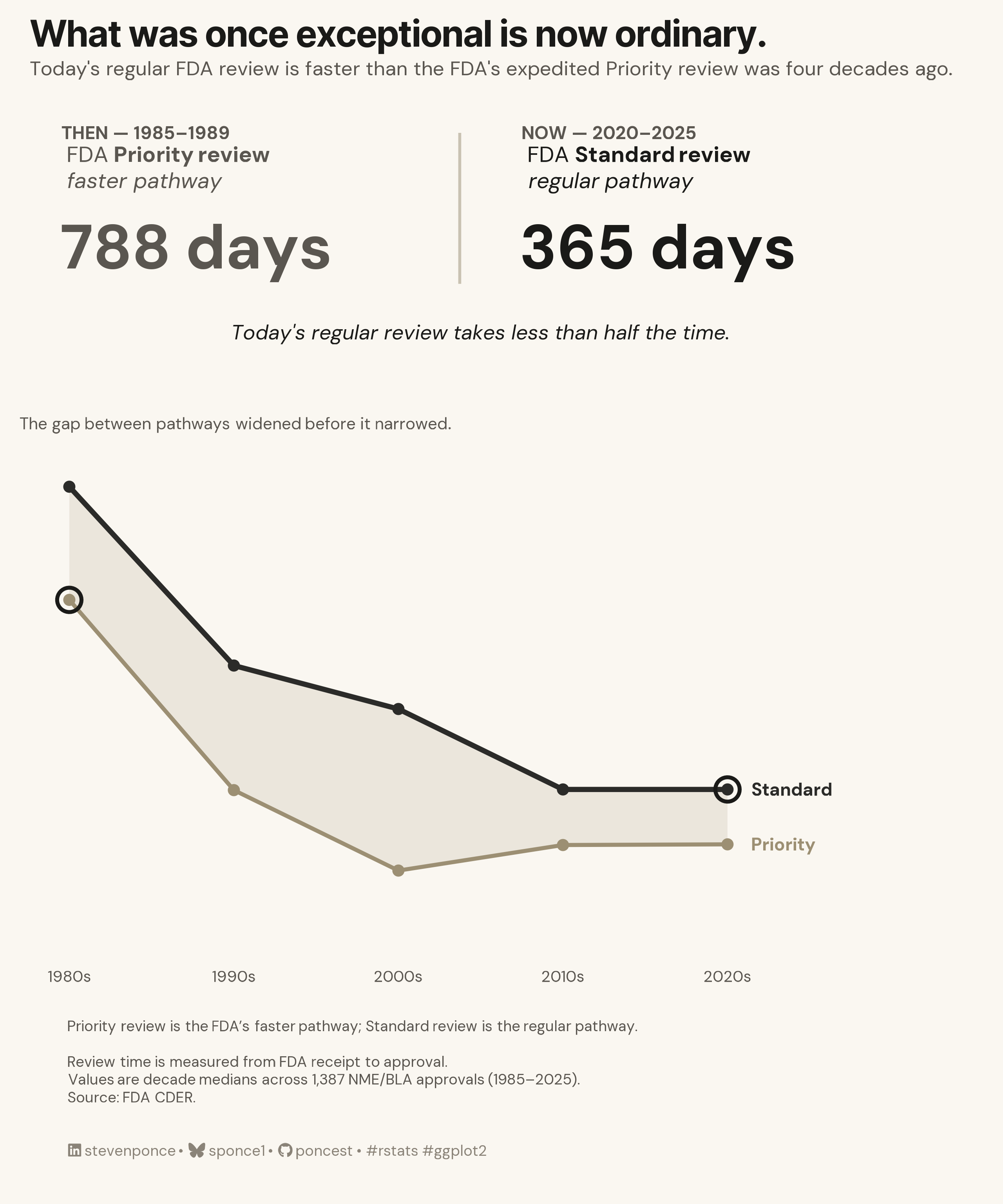
FDA drug review times fell across the board from 1985 to 2025, but the sharpest gains came from the collapse of the Priority pathway’s once-widening advantage over Standard review. Built from 1,387 NME/BLA approvals using decade-median comparisons, with a cross-era THEN/NOW framing rather than a raw distribution chart. Created in R with ggplot2, patchwork, and ggtext.

Figure 1: Editorial infographic titled “What was once exceptional is now ordinary.” A 1980s FDA Priority review took a median of 788 days; a 2020s FDA Standard review takes 365 days — less than half the time. A line chart below shows median review days by decade, 1985–2025, for both pathways: Priority stayed faster throughout, but its advantage over Standard widened through the 1990s–2000s before narrowing sharply after 2010. Based on 1,387 NME/BLA approvals. Source: FDA CDER.

Steps to Create this Graphic

1. Load Packages & Setup

```{r}
#| label: load
#| warning: false
#| message: false      
#| results: "hide"     

## 1. LOAD PACKAGES & SETUP ----
suppressPackageStartupMessages({
if (!require("pacman")) install.packages("pacman")
pacman::p_load(
    tidyverse, ggtext, showtext, janitor, patchwork,
    scales, glue, here
    )
})

### |- figure size ----          
camcorder::gg_record(
    dir    = here::here("temp_plots"),
    device = "png",
    width  = 8,
    height = 9.6,
    units  = "in",
    dpi    = 320
)

# Source utility functions
suppressMessages(source(here::here("R/utils/fonts.R")))
source(here::here("R/utils/social_icons.R"))
source(here::here("R/utils/image_utils.R"))
source(here::here("R/themes/base_theme.R"))
```

2. Read in the Data

```{r}
#| label: read
#| include: true
#| eval: true
#| warning: false

raw <- read_csv(
  here::here("data/nme_approvals_raw.csv"), show_col_types = FALSE) |>
  clean_names()
```

3. Examine the Data

```{r}
#| label: examine
#| include: true
#| eval: true
#| results: 'hide'
#| warning: false

glimpse(raw)
```

4. Tidy Data

```{r}
#| label: tidy
#| warning: false

nme <- raw |>
  mutate(
    receipt_date = mdy(fda_receipt_date),
    approval_date = mdy(fda_approval_date),
    review_days = as.numeric(approval_date - receipt_date),
    decade = paste0(floor(approval_year / 10) * 10, "s"),
    rd = if_else(str_starts(review_designation, "Priority"),
      "Priority", "Standard"
    )
  ) |>
  filter(!is.na(review_days), review_days >= 0)

decade_levels <- c("1980s", "1990s", "2000s", "2010s", "2020s")

medians <- nme |>
  group_by(decade, rd) |>
  summarise(median_days = median(review_days), n = n(), .groups = "drop") |>
  mutate(decade = factor(decade, levels = decade_levels)) |>
  arrange(decade)

HERO_PRIORITY_80S <- medians |>
  filter(decade == "1980s", rd == "Priority") |>
  pull(median_days)

HERO_STANDARD_20S <- medians |>
  filter(decade == "2020s", rd == "Standard") |>
  pull(median_days)
```

5. Visualization Parameters

```{r}
#| label: params
#| include: true
#| warning: false

### |-  plot aesthetics ----
colors <- get_theme_colors(
  palette = c(
    bg        = "#FAF7F1",
    charcoal  = "#2B2B29",
    priority  = "#9C8F73",
    text      = "#1A1A18",
    subtext   = "#5A5650",
    ring      = "#1A1A18",
    refline   = "#C9C2B2"
  )
)

### |-  fonts ----
setup_fonts()
fonts <- get_font_families()

font_add_google("Inter Tight", "inter_tight_title")
showtext_auto()
```

6. Plot

```{r}
#| label: plot
#| warning: false

### |- hero panel: THEN / NOW ----
hero <- ggplot() +
  xlim(0, 1) +
  ylim(0, 1) +
  annotate("segment",
    x = 0.475, xend = 0.475, y = 0.42, yend = 0.95,
    color = colors$palette["refline"], linewidth = 0.8
  ) +
  annotate("text",
    x = 0.0, y = 0.95, label = "THEN \u2014 1985\u20131989",
    hjust = 0, size = 3.6, family = fonts$text, fontface = "bold",
    color = colors$palette["subtext"]
  ) +
  annotate("richtext",
    x = 0.0, y = 0.82,
    label = "FDA **Priority review**<br><i>faster pathway</i>",
    hjust = 0, size = 4.4, family = fonts$text, color = colors$palette["subtext"],
    fill = NA, label.color = NA
  ) +
  annotate("text",
    x = 0.0, y = 0.55, label = glue("{HERO_PRIORITY_80S} days"),
    hjust = 0, size = 12.5, family = fonts$text, fontface = "bold",
    color = colors$palette["subtext"]
  ) +
  annotate("text",
    x = 0.55, y = 0.95, label = "NOW \u2014 2020\u20132025",
    hjust = 0, size = 3.6, family = fonts$text, fontface = "bold",
    color = colors$palette["subtext"]
  ) +
  annotate("richtext",
    x = 0.55, y = 0.82,
    label = "FDA **Standard review**<br><i>regular pathway</i>",
    hjust = 0, size = 4.4, family = fonts$text, color = colors$palette["text"],
    fill = NA, label.color = NA
  ) +
  annotate("text",
    x = 0.55, y = 0.55, label = glue("{HERO_STANDARD_20S} days"),
    hjust = 0, size = 12.5, family = fonts$text, fontface = "bold",
    color = colors$palette["text"]
  ) +
  annotate("text",
    x = 0.5, y = 0.25,
    label = "Today's regular review takes less than half the time.",
    hjust = 0.5, size = 4.2, family = fonts$text, color = colors$palette["text"],
    fontface = "italic"
  ) +
  theme_void() +
  theme(plot.background = element_rect(fill = colors$palette["bg"], color = NA))

### |- supporting evidence panel ----
med_wide <- medians |>
  select(decade, rd, median_days) |>
  pivot_wider(names_from = rd, values_from = median_days)

label_df <- med_wide |> filter(decade == "2020s")

ring_points <- medians |>
  filter((decade == "1980s" & rd == "Priority") |
    (decade == "2020s" & rd == "Standard"))

evidence <- ggplot(medians, aes(x = decade, y = median_days, group = rd)) +
  geom_ribbon(
    data = med_wide, aes(x = decade, ymin = Priority, ymax = Standard, group = 1),
    inherit.aes = FALSE, fill = colors$palette["priority"], alpha = 0.16
  ) +
  geom_line(aes(color = rd, linewidth = rd)) +
  geom_point(aes(color = rd), size = 2.6) +
  geom_point(
    data = ring_points, color = colors$palette["ring"], size = 5.5,
    shape = 21, stroke = 1.6, fill = NA
  ) +
  geom_text(
    data = label_df |> pivot_longer(c(Priority, Standard),
      names_to = "rd", values_to = "median_days"
    ),
    aes(x = 5.15, y = median_days, label = rd, color = rd),
    hjust = 0, size = 3.6, family = fonts$text, fontface = "bold",
    inherit.aes = FALSE
  ) +
  scale_color_manual(
    values = c(Priority = "#9C8F73", Standard = "#2B2B29"),
    guide = "none"
  ) +
  scale_linewidth_manual(values = c(Priority = 1.1, Standard = 1.4), guide = "none") +
  scale_x_discrete(expand = expansion(add = c(0.3, 1.3))) +
  scale_y_continuous(limits = c(0, NA), expand = expansion(mult = c(0.02, 0.1))) +
  labs(
    title = "The gap between pathways widened before it narrowed.",
    x = NULL, y = NULL
  ) +
  theme_minimal(base_family = fonts$text) +
  theme(
    plot.background = element_rect(fill = colors$palette["bg"], color = NA),
    panel.background = element_rect(fill = colors$palette["bg"], color = NA),
    panel.grid = element_blank(),
    axis.text.x = element_text(size = 9, color = colors$palette["subtext"]),
    axis.text.y = element_blank(),
    plot.title = element_textbox_simple(
      size = 9.5, color = colors$palette["subtext"], margin = margin(b = 4), width = unit(1, "npc")
    ),
    plot.margin = margin(0, 30, 0, 6)
  )

### |- footer ----
footer_text <- str_glue(
  "Priority review is the FDA's faster pathway; Standard review is the regular pathway.<br><br>",
  "Review time is measured from FDA receipt to approval.<br>",
  "Values are decade medians across 1,387 NME/BLA approvals (1985\u20132025).<br>",
  "Source: FDA CDER."
)

icons <- get_social_icons()

caption_text <- str_glue(
  "{footer_text}<br><br><br>",
  "<span style='color:#8A8378'>{icons$linkedin} stevenponce &bull; {icons$bluesky} sponce1 &bull; ",
  "{icons$github} poncest &bull; #rstats #ggplot2</span>"
)

footer <- ggplot() +
  annotate("richtext",
    x = 0, y = 0, label = caption_text,
    hjust = 0, size = 3, family = fonts$text, color = colors$palette["subtext"],
    fill = NA, label.color = NA
  ) +
  xlim(0, 1) +
  ylim(-0.45, 0.45) +
  theme_void() +
  theme(plot.background = element_rect(fill = colors$palette["bg"], color = NA))

### |- compose ----
final_plot <- hero / evidence / footer +
  plot_layout(heights = c(1.2, 2.0, 0.8)) +
  plot_annotation(
    title = "What was once exceptional is now ordinary.",
    subtitle = "Today's regular FDA review is faster than the FDA's expedited Priority review was four decades ago.",
    theme = theme(
      plot.background = element_rect(fill = colors$palette["bg"], color = NA),
      plot.title = element_text(
        family = "inter_tight_title", face = "bold", size = 21,
        color = colors$palette["text"], margin = margin(6, 0, 4, 6)
      ),
      plot.subtitle = element_text(
        family = fonts$text, size = 11.5, color = colors$palette["subtext"],
        margin = margin(0, 0, 14, 6)
      )
    )
  ) &
  theme(plot.background = element_rect(fill = colors$palette["bg"], color = NA))
```

7. Save

```{r}
#| label: save
#| warning: false

### |-  plot image ----

main_file <- here::here("projects/standalone_visualizations/sa_2026-07-24.png")
thumb_file <- here::here("projects/standalone_visualizations/thumbnails/sa_2026-07-24.png")

dir.create(dirname(main_file), recursive = TRUE, showWarnings = FALSE)
dir.create(dirname(thumb_file), recursive = TRUE, showWarnings = FALSE)

latest_frame <- list.files(here::here("temp_plots"), full.names = TRUE) |>
  (\(f) f[order(file.info(f)$mtime)])() |>
  tail(1)

file.copy(from = latest_frame, to = main_file, overwrite = TRUE)

magick::image_read(main_file) |>
  magick::image_resize("400") |>
  magick::image_write(thumb_file)
```

[1] TRUE

8. Session Info

TipExpand for Session Info

R version 4.6.1 (2026-06-24)
Platform: aarch64-apple-darwin23
Running under: macOS Tahoe 26.5.2

Matrix products: default
BLAS:   /Library/Frameworks/R.framework/Versions/4.6/Resources/lib/libRblas.0.dylib 
LAPACK: /Library/Frameworks/R.framework/Versions/4.6/Resources/lib/libRlapack.dylib;  LAPACK version 3.12.1

locale:
[1] en_US.UTF-8/en_US.UTF-8/en_US.UTF-8/C/en_US.UTF-8/en_US.UTF-8

time zone: America/New_York
tzcode source: internal

attached base packages:
[1] stats     graphics  grDevices utils     datasets  methods   base     

other attached packages:
 [1] here_1.0.2      glue_1.8.1      scales_1.4.0    patchwork_1.3.2
 [5] janitor_2.2.1   showtext_0.9-8  showtextdb_3.0  sysfonts_0.8.9 
 [9] ggtext_0.1.2    lubridate_1.9.5 forcats_1.0.1   stringr_1.6.0  
[13] dplyr_1.2.1     purrr_1.2.2     readr_2.2.0     tidyr_1.3.2    
[17] tibble_3.3.1    ggplot2_4.0.3   tidyverse_2.0.0 pacman_0.5.1   

loaded via a namespace (and not attached):
 [1] gtable_0.3.6       xfun_0.60          htmlwidgets_1.6.4  tzdb_0.5.0        
 [5] vctrs_0.7.3        tools_4.6.1        generics_0.1.4     curl_7.1.0        
 [9] parallel_4.6.1     gifski_1.32.0-2    pkgconfig_2.0.3    RColorBrewer_1.1-3
[13] S7_0.2.2           lifecycle_1.0.5    compiler_4.6.1     farver_2.1.2      
[17] textshaping_1.0.5  codetools_0.2-20   snakecase_0.11.1   htmltools_0.5.9   
[21] yaml_2.3.12        pillar_1.11.1      crayon_1.5.3       camcorder_0.1.0   
[25] magick_2.9.1       tidyselect_1.2.1   digest_0.6.39      stringi_1.8.7     
[29] rsvg_2.7.0         rprojroot_2.1.1    fastmap_1.2.0      grid_4.6.1        
[33] cli_3.6.6          magrittr_2.0.5     withr_3.0.3        bit64_4.8.2       
[37] timechange_0.4.0   rmarkdown_2.31     bit_4.6.0          otel_0.2.0        
[41] hms_1.1.4          evaluate_1.0.5     knitr_1.51         rlang_1.3.0       
[45] gridtext_0.1.6     Rcpp_1.1.2         xml2_1.6.0         svglite_2.2.2     
[49] rstudioapi_0.19.0  vroom_1.7.1        jsonlite_2.0.0     R6_2.6.1          
[53] systemfonts_1.3.2 

9. GitHub Repository

TipExpand for GitHub Repo

The complete code for this analysis is available in sa_2026-07-24.qmd.

For the full repository, click here.

10. References

TipExpand for References

1. Data Source:
   • U.S. Food and Drug Administration, CDER: Compilation of CDER New Molecular Entity (NME) Drug and New Biologic Approvals
   • Data pulled 2026-07-18. The FDA updates this page as new approvals occur; figures reflect approvals recorded as of the pull date, not the current state of the source page.

11. Custom Functions Documentation

Note📦 Custom Helper Functions

This analysis uses custom functions from my personal module library for efficiency and consistency across projects.

Functions Used:

• fonts.R: setup_fonts(), get_font_families() - Font management with showtext
• social_icons.R: create_social_caption() - Generates formatted social media captions
• image_utils.R: save_plot() - Consistent plot saving with naming conventions
  • ⚠️ save_plot_patchwork() has a known reliability issue when called from a Quarto .qmd render alongside camcorder::gg_record() — the two appear to conflict over graphics device state, causing a dev.off() failure that masks the real underlying error. This piece uses plain ggsave() + manual thumbnail generation instead. Confirmed via a prior standalone project hitting the same root cause.
• base_theme.R: create_base_theme(), extend_weekly_theme(), get_theme_colors() - Custom ggplot2 themes

Why custom functions?
These utilities standardize theming, fonts, and output across all my data visualizations. The core analysis (data tidying and visualization logic) uses only standard tidyverse packages.

Source Code:
View all custom functions → GitHub: R/utils