• Steven Ponce
  • About
  • Data Visualizations
  • Projects
  • Resume
  • Email

On this page

  • Steps to Create this Graphic
    • 1. Load Packages & Setup
    • 2. Read in the Data
    • 3. Examine the Data
    • 4. Tidy Data
    • 5. Visualization Parameters
    • 6. Plot
    • 7. Save
    • 8. Session Info
    • 9. GitHub Repository
    • 10. References
    • 11. Custom Functions Documentation

One Intervention, System-Wide Impact

  • Show All Code
  • Hide All Code

  • View Source

Wolf reintroduction triggered a trophic cascade across Yellowstone’s ecosystem.

30DayChartChallenge
Data Visualization
R Programming
2026
A vertical trophic cascade diagram showing how wolf reintroduction in Yellowstone in 1995 triggered system-wide ecological recovery across five interdependent levels — from apex predator to river systems. Built with ggplot2 using curated directional indices based on Ripple & Beschta (2012).
Author

Steven Ponce

Published

April 13, 2026

Figure 1: A vertical node-arrow diagram titled “One Intervention, System-Wide Impact.” Five trophic levels cascade top to bottom: Wolves (apex predator, index 0 to 100), Elk (herbivore, 100 to 40), Willows (vegetation, 20 to 80), Beavers (engineer, 5 to 25), and Rivers (landscape, 30 to 70). A red arrow connects Wolves to Elk, labeled “elk population declined, movement patterns shifted.” Three green arrows follow, each labeled with a recovery effect: overgrazing was reduced and vegetation recovered; willow thickets expanded and beaver habitat was restored; beaver dams increased, and rivers stabilized. An intervention callout marks 1995 as the year wolves were reintroduced to Yellowstone. A result box at the bottom reads: Rivers stabilized, Biodiversity increased, Ecosystem resilience restored. Data source: Ripple and Beschta (2012); values are directional indices, not absolute counts.

Steps to Create this Graphic

1. Load Packages & Setup

Show code
```{r}
#| label: load
#| warning: false
#| message: false      
#| results: "hide"     

## 1. LOAD PACKAGES & SETUP ----
suppressPackageStartupMessages({
pacman::p_load(
  tidyverse, ggtext, showtext,  
  janitor, scales, glue
  )
})

### |- figure size ----
camcorder::gg_record(
  dir    = here::here("temp_plots"),
  device = "png",
  width  = 10,
  height = 8,
  units  = "in",
  dpi    = 320
)

# Source utility functions
suppressMessages(source(here::here("R/utils/fonts.R")))
source(here::here("R/utils/social_icons.R"))
source(here::here("R/utils/image_utils.R"))
source(here::here("R/themes/base_theme.R"))
```

2. Read in the Data

Show code
```{r}
#| label: read
#| include: true
#| eval: true
#| warning: false

### |- trophic nodes ----
# Each entity = one level in the Yellowstone cascade
# y positions are fixed for vertical layout (top → bottom)
nodes <- tribble(
  ~entity,    ~trophic_level,  ~y,  ~before, ~after,  ~direction,
  "Wolves",   "Apex Predator", 4.0,       0,    100,  "restored",
  "Elk",      "Herbivore",     3.0,     100,     40,  "reduced",
  "Willows",  "Vegetation",    2.0,      20,     80,  "recovered",
  "Beavers",  "Engineer",      1.0,       5,     25,  "recovered",
  "Rivers",   "Landscape",     0.0,      30,     70,  "stabilized"
)

### |- arrows (edges) ----,
# Each row = one causal link between consecutive trophic levels
# label = annotation text on the arrow
# effect = positive or negative pressure
edges <- tribble(
  ~from,      ~to,        ~y_from, ~y_to, ~effect,    ~label,
  "Wolves",   "Elk",          5.0,   3.8, "negative", "elk population declined\nmovement patterns shifted",
  "Elk",      "Willows",      3.8,   2.6, "positive", "overgrazing reduced\nvegetation recovered",
  "Willows",  "Beavers",      2.6,   1.4, "positive", "willow thickets expanded\nbeaver habitat restored",
  "Beavers",  "Rivers",       1.4,   0.2, "positive", "beaver dams increased\nrivers stabilized"
)
```

3. Examine the Data

Show code
```{r}
#| label: examine
#| include: true
#| eval: true
#| results: 'hide'
#| warning: false

glimpse(nodes)
```

4. Tidy Data

Show code
```{r}
#| label: tidy
#| warning: false

### |- x positions ----
x_node        <-  0.0
x_seg         <-  0.0     
x_label_right <-  0.28    
x_left        <- -0.88    
node_r <- 0.38
```

5. Visualization Parameters

Show code
```{r}
#| label: params
#| include: true
#| warning: false

### |- plot aesthetics ----
colors <- get_theme_colors(
  palette = list(
    col_wolf      = "#8B1A1A",   
    col_elk       = "#C0392B",   
    col_recovered = "#2E7D32",   
    col_neutral   = "#455A64",   
    col_arrow_neg = "#C0392B",   
    col_arrow_pos = "#1B5E20",   
    col_label_bg  = "#FFFFFF",
    bg_color      = "#FAFAF7",
    text_color    = "#1C1C1C",
    grid_color    = "#E8E8E4"
  )
)

### |- node color assignment ----
nodes <- nodes |>
  mutate(
    node_color = case_when(
      entity == "Wolves"  ~ colors$palette$col_wolf,
      entity == "Elk"     ~ colors$palette$col_elk,
      TRUE                ~ colors$palette$col_recovered
    ),
    node_color_text = case_when(
      entity == "Wolves"  ~ colors$palette$col_wolf,
      entity == "Elk"     ~ colors$palette$col_elk,
      TRUE                ~ colors$palette$col_recovered
    ),
    node_fill = case_when(
      entity == "Wolves"  ~ "#FFF0F0",
      entity == "Elk"     ~ "#FFF5F5",
      TRUE                ~ "#F1F8F1"
    )
  )

edges <- edges |>
  mutate(
    y_from = case_when(
      from == "Wolves"  ~ 4.0,
      from == "Elk"     ~ 3.0,
      from == "Willows" ~ 2.0,
      from == "Beavers" ~ 1.0
    ),
    y_to = case_when(
      to == "Elk"     ~ 3.0,
      to == "Willows" ~ 2.0,
      to == "Beavers" ~ 1.0,
      to == "Rivers"  ~ 0.0
    ),
    arrow_color = if_else(
      effect == "negative", 
      colors$palette$col_arrow_neg, 
      colors$palette$col_arrow_pos)
  )

### |- titles and caption ----
title_text    <- "One Intervention, System-Wide Impact"

subtitle_text <- "Wolf reintroduction triggered a trophic cascade across Yellowstone's ecosystem."

caption_text  <- create_dcc_caption(
  dcc_year    = 2026,
  dcc_day     = 13,
  source_text = "Ripple & Beschta (2012); Beschta & Ripple (2009)<br>Values are directional indices, not absolute counts"
)

### |- fonts ----
setup_fonts()
fonts <- get_font_families()
```

6. Plot

Show code
```{r}
#| label: plot
#| warning: false

### |- main plot ----
p <- ggplot() +

  # trophic level labels
  geom_text(
    data = nodes,
    aes(x = x_left, y = y + 0.18, label = str_to_upper(trophic_level)),
    hjust = 0,
    vjust = 1,
    size = 2.2,
    color = "#888888",
    family = fonts$text,
    fontface = "plain"
  ) +
  # before/after index 
  geom_text(
    data = nodes,
    aes(
      x = x_left, y = y - 0.04,
      label = glue("{before} to {after}"),
      color = I(node_color)
    ),
    hjust = 0,
    vjust = 1,
    size = 2.9,
    family = fonts$text,
    fontface = "bold"
  ) +
  # straight arrow segments 
  geom_segment(
    data = edges,
    aes(
      y     = y_from - node_r,
      yend  = y_to + node_r,
      color = I(arrow_color)
    ),
    x = 0,
    xend = 0,
    linewidth = 1.5,
    arrow = arrow(length = unit(0.18, "inches"), type = "closed", ends = "last"),
    lineend = "butt"
  ) +
  # edge annotation labels
  geom_label(
    data = edges,
    aes(
      x     = x_label_right,
      y     = (y_from + y_to) / 2,
      label = label,
      color = I(arrow_color)
    ),
    hjust = 0,
    vjust = 0.5,
    size = 2.9,
    family = fonts$text,
    fontface = "italic",
    fill = colors$palette$col_label_bg,
    linewidth = 0,
    label.padding = unit(0.18, "lines"),
    lineheight = 1.3
  ) +
  # node circles
  geom_point(
    data = nodes,
    aes(y = y, color = I(node_color), fill = I(node_fill)),
    x = 0,
    size = 17,
    shape = 21,
    stroke = 2.0
  ) +
  # node entity labels 
  geom_text(
    data = nodes,
    aes(y = y, label = entity, color = I(node_color)),
    x = 0,
    size = 3.1,
    family = fonts$text,
    fontface = "bold"
  ) +
  # "INDEX" column header
  annotate(
    "text",
    x = x_left, y = 4.40,
    label = "INDEX: before vs. after",
    hjust = 0,
    vjust = 1,
    size = 2.2,
    color = "#AAAAAA",
    family = fonts$text
  ) +
  # intervention callout 
  annotate(
    "label",
    x = 0, y = 4.44,
    label = "1995: Wolves reintroduced to Yellowstone",
    hjust = 0.5,
    vjust = 0,
    size = 3.0,
    color = colors$palette$col_wolf,
    fill = "#FFF5F5",
    linewidth = 0.3,
    family = fonts$text,
    fontface = "bold"
  ) +
  # outcome callout
  annotate(
    "label",
    x = 0, y = -0.45,
    label = "Result: Rivers stabilized  |  Biodiversity increased  |  Ecosystem resilience restored",
    hjust = 0.5,
    vjust = 1,
    size = 2.8,
    color = colors$palette$col_recovered,
    fill = "#F1F8F1",
    linewidth = 0.3,
    family = fonts$text
  ) +
  # scales
  scale_x_continuous(limits = c(-1.05, 1)) +
  scale_y_continuous(limits = c(-0.72, 4.75)) +
  # labs 
  labs(
    title    = title_text,
    subtitle = subtitle_text,
    caption  = caption_text
  ) +
  # theme 
  theme_void() +
  theme(
    plot.background = element_rect(fill = colors$palette$bg_color, color = NA),
    panel.background = element_rect(fill = colors$palette$bg_color, color = NA),
    plot.title = element_text(
      family = fonts$title, face = "bold",
      size = 26, color = colors$palette$text_color,
      margin = margin(t = 10, b = 6, l = 5)
    ),
    plot.subtitle = element_textbox_simple(
      family = fonts$text,
      size = 11,
      color = "#444444",
      lineheight = 1.3,
      margin = margin(t = 5, b = 8, l = 5)
    ),
    plot.caption = element_textbox_simple(
      family = fonts$text,
      size = 7.5,
      color = "#888888",
      lineheight = 1.3,
      margin = margin(t = 8, b = 6)
    ),
    plot.margin = margin(t = 20, r = 20, b = 12, l = 20)
  )
```

7. Save

Show code
```{r}
#| label: save
#| warning: false

### |-  plot image ----  
save_plot(
  p, 
  type = "30daychartchallenge", 
  year = 2026, 
  day = 13, 
  width = 8, 
  height = 10
  )
```

8. Session Info

TipExpand for Session Info
R version 4.3.1 (2023-06-16 ucrt)
Platform: x86_64-w64-mingw32/x64 (64-bit)
Running under: Windows 11 x64 (build 26100)

Matrix products: default


locale:
[1] LC_COLLATE=English_United States.utf8 
[2] LC_CTYPE=English_United States.utf8   
[3] LC_MONETARY=English_United States.utf8
[4] LC_NUMERIC=C                          
[5] LC_TIME=English_United States.utf8    

time zone: America/New_York
tzcode source: internal

attached base packages:
[1] stats     graphics  grDevices utils     datasets  methods   base     

other attached packages:
 [1] here_1.0.2      glue_1.8.0      scales_1.4.0    janitor_2.2.1  
 [5] showtext_0.9-7  showtextdb_3.0  sysfonts_0.8.9  ggtext_0.1.2   
 [9] lubridate_1.9.5 forcats_1.0.1   stringr_1.6.0   dplyr_1.2.0    
[13] purrr_1.2.1     readr_2.2.0     tidyr_1.3.2     tibble_3.2.1   
[17] ggplot2_4.0.2   tidyverse_2.0.0

loaded via a namespace (and not attached):
 [1] gtable_0.3.6       xfun_0.56          htmlwidgets_1.6.4  tzdb_0.5.0        
 [5] vctrs_0.7.1        tools_4.3.1        generics_0.1.4     curl_7.0.0        
 [9] gifski_1.32.0-2    pacman_0.5.1       pkgconfig_2.0.3    RColorBrewer_1.1-3
[13] S7_0.2.0           lifecycle_1.0.5    compiler_4.3.1     farver_2.1.2      
[17] textshaping_1.0.4  codetools_0.2-19   snakecase_0.11.1   litedown_0.9      
[21] htmltools_0.5.9    yaml_2.3.12        pillar_1.11.1      camcorder_0.1.0   
[25] magick_2.8.6       commonmark_2.0.0   tidyselect_1.2.1   digest_0.6.39     
[29] stringi_1.8.7      labeling_0.4.3     rsvg_2.6.2         rprojroot_2.1.1   
[33] fastmap_1.2.0      grid_4.3.1         cli_3.6.5          magrittr_2.0.3    
[37] withr_3.0.2        timechange_0.4.0   rmarkdown_2.30     otel_0.2.0        
[41] ragg_1.5.0         hms_1.1.4          evaluate_1.0.5     knitr_1.51        
[45] markdown_2.0       rlang_1.1.7        gridtext_0.1.6     Rcpp_1.1.1        
[49] xml2_1.5.2         svglite_2.1.3      rstudioapi_0.18.0  jsonlite_2.0.0    
[53] R6_2.6.1           systemfonts_1.3.2 

9. GitHub Repository

TipExpand for GitHub Repo

The complete code for this analysis is available in 30dcc_2026_13.qmd.

For the full repository, click here.

10. References

TipExpand for References
  1. Data Sources:
    • Ripple, W. J., & Beschta, R. L. (2012). Trophic cascades in Yellowstone: The first 15 years after wolf reintroduction. Biological Conservation, 145(1), 205–213. https://doi.org/10.1016/j.biocon.2011.11.005
    • Beschta, R. L., & Ripple, W. J. (2009). Large predators and trophic cascades in terrestrial ecosystems of the western United States. Biological Conservation, 142(11), 2401–2414. https://doi.org/10.1016/j.biocon.2009.06.015
    • Hebblewhite, M., White, C. A., Nietvelt, C. G., McKenzie, J. A., Hurd, T. E., Fryxell, J. M., Bayley, S. E., & Paquet, P. C. (2005). Human activity mediates a trophic cascade caused by wolves. Ecology, 86(8), 2135–2144. https://doi.org/10.1890/04-1269
  2. Note: Index values (0–100) are directional and illustrative, constructed to reflect relative magnitude of change as reported in the literature above. They are not absolute population counts or official measurements.

11. Custom Functions Documentation

Note📦 Custom Helper Functions

This analysis uses custom functions from my personal module library for efficiency and consistency across projects.

Functions Used:

  • fonts.R: setup_fonts(), get_font_families() - Font management with showtext
  • social_icons.R: create_social_caption() - Generates formatted social media captions
  • image_utils.R: save_plot() - Consistent plot saving with naming conventions
  • base_theme.R: create_base_theme(), extend_weekly_theme(), get_theme_colors() - Custom ggplot2 themes

Why custom functions?
These utilities standardize theming, fonts, and output across all my data visualizations. The core analysis (data tidying and visualization logic) uses only standard tidyverse packages.

Source Code:
View all custom functions → GitHub: R/utils

Back to top

Citation

BibTeX citation:
@online{ponce2026,
  author = {Ponce, Steven},
  title = {One {Intervention,} {System-Wide} {Impact}},
  date = {2026-04-13},
  url = {https://stevenponce.netlify.app/data_visualizations/30DayChartChallenge/2026/30dcc_2026_13.html},
  langid = {en}
}
For attribution, please cite this work as:
Ponce, Steven. 2026. “One Intervention, System-Wide Impact.” April 13, 2026. https://stevenponce.netlify.app/data_visualizations/30DayChartChallenge/2026/30dcc_2026_13.html.
Source Code
---
title: "One Intervention, System-Wide Impact"
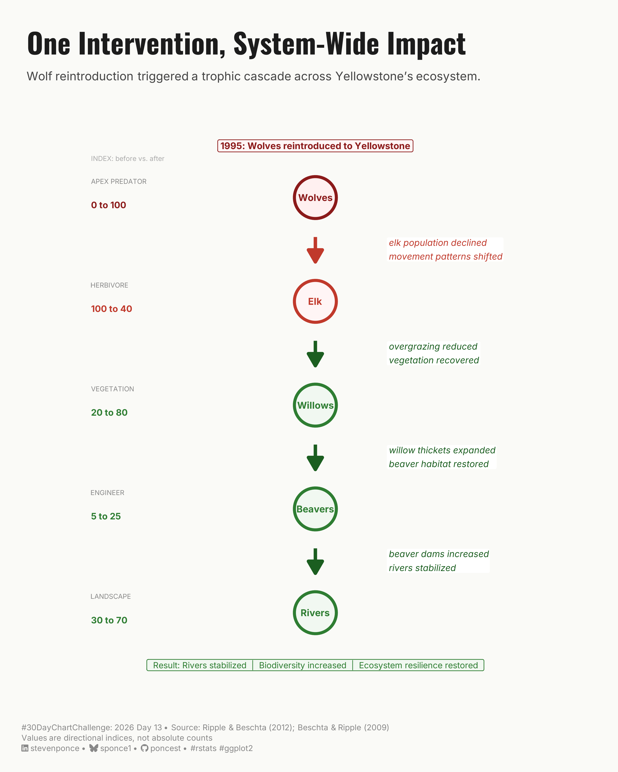
subtitle: "Wolf reintroduction triggered a trophic cascade across Yellowstone's ecosystem."
description: "A vertical trophic cascade diagram showing how wolf reintroduction in Yellowstone in 1995 triggered system-wide ecological recovery across five interdependent levels — from apex predator to river systems. Built with ggplot2 using curated directional indices based on Ripple & Beschta (2012)."
date: "2026-04-13" 
author:
  - name: "Steven Ponce"
    url: "https://stevenponce.netlify.app"
citation:
  url: "https://stevenponce.netlify.app/data_visualizations/30DayChartChallenge/2026/30dcc_2026_13.html"
categories: ["30DayChartChallenge", "Data Visualization", "R Programming", "2026"]
tags: [
  "30DayChartChallenge",
  "Relationships",
  "Ecosystems",
  "Trophic Cascade",
  "Node-Arrow Diagram",
  "Yellowstone",
  "Wolf Reintroduction",
  "Ecology",
  "Causal Diagram",
  "System Diagram",
  "ggplot2",
  "Annotated Chart",
  "Conservation"
]
image: "thumbnails/30dcc_2026_13.png"
format:
  html:
    toc: true
    toc-depth: 5
    code-link: true
    code-fold: true
    code-tools: true
    code-summary: "Show code"
    self-contained: true
    theme: 
      light: [flatly, assets/styling/custom_styles.scss]
      dark: [darkly, assets/styling/custom_styles_dark.scss]
editor_options: 
  chunk_output_type: inline
execute: 
  freeze: true                                                  
  cache: true                                                   
  error: false
  message: false
  warning: false
  eval: true
---

![A vertical node-arrow diagram titled "One Intervention, System-Wide Impact." Five trophic levels cascade top to bottom: Wolves (apex predator, index 0 to 100), Elk (herbivore, 100 to 40), Willows (vegetation, 20 to 80), Beavers (engineer, 5 to 25), and Rivers (landscape, 30 to 70). A red arrow connects Wolves to Elk, labeled "elk population declined, movement patterns shifted." Three green arrows follow, each labeled with a recovery effect: overgrazing was reduced and vegetation recovered; willow thickets expanded and beaver habitat was restored; beaver dams increased, and rivers stabilized. An intervention callout marks 1995 as the year wolves were reintroduced to Yellowstone. A result box at the bottom reads: Rivers stabilized, Biodiversity increased, Ecosystem resilience restored. Data source: Ripple and Beschta (2012); values are directional indices, not absolute counts.](30dcc_2026_13.png){#fig-1}

### [**Steps to Create this Graphic**]{.mark}

#### [1. Load Packages & Setup]{.smallcaps}

```{r}
#| label: load
#| warning: false
#| message: false      
#| results: "hide"     

## 1. LOAD PACKAGES & SETUP ----
suppressPackageStartupMessages({
pacman::p_load(
  tidyverse, ggtext, showtext,  
  janitor, scales, glue
  )
})

### |- figure size ----
camcorder::gg_record(
  dir    = here::here("temp_plots"),
  device = "png",
  width  = 10,
  height = 8,
  units  = "in",
  dpi    = 320
)

# Source utility functions
suppressMessages(source(here::here("R/utils/fonts.R")))
source(here::here("R/utils/social_icons.R"))
source(here::here("R/utils/image_utils.R"))
source(here::here("R/themes/base_theme.R"))
```

#### [2. Read in the Data]{.smallcaps}

```{r}
#| label: read
#| include: true
#| eval: true
#| warning: false

### |- trophic nodes ----
# Each entity = one level in the Yellowstone cascade
# y positions are fixed for vertical layout (top → bottom)
nodes <- tribble(
  ~entity,    ~trophic_level,  ~y,  ~before, ~after,  ~direction,
  "Wolves",   "Apex Predator", 4.0,       0,    100,  "restored",
  "Elk",      "Herbivore",     3.0,     100,     40,  "reduced",
  "Willows",  "Vegetation",    2.0,      20,     80,  "recovered",
  "Beavers",  "Engineer",      1.0,       5,     25,  "recovered",
  "Rivers",   "Landscape",     0.0,      30,     70,  "stabilized"
)

### |- arrows (edges) ----,
# Each row = one causal link between consecutive trophic levels
# label = annotation text on the arrow
# effect = positive or negative pressure
edges <- tribble(
  ~from,      ~to,        ~y_from, ~y_to, ~effect,    ~label,
  "Wolves",   "Elk",          5.0,   3.8, "negative", "elk population declined\nmovement patterns shifted",
  "Elk",      "Willows",      3.8,   2.6, "positive", "overgrazing reduced\nvegetation recovered",
  "Willows",  "Beavers",      2.6,   1.4, "positive", "willow thickets expanded\nbeaver habitat restored",
  "Beavers",  "Rivers",       1.4,   0.2, "positive", "beaver dams increased\nrivers stabilized"
)

```

#### [3. Examine the Data]{.smallcaps}

```{r}
#| label: examine
#| include: true
#| eval: true
#| results: 'hide'
#| warning: false

glimpse(nodes)
```

#### [4. Tidy Data]{.smallcaps}

```{r}
#| label: tidy
#| warning: false

### |- x positions ----
x_node        <-  0.0
x_seg         <-  0.0     
x_label_right <-  0.28    
x_left        <- -0.88    
node_r <- 0.38
```


#### [5. Visualization Parameters]{.smallcaps}

```{r}
#| label: params
#| include: true
#| warning: false

### |- plot aesthetics ----
colors <- get_theme_colors(
  palette = list(
    col_wolf      = "#8B1A1A",   
    col_elk       = "#C0392B",   
    col_recovered = "#2E7D32",   
    col_neutral   = "#455A64",   
    col_arrow_neg = "#C0392B",   
    col_arrow_pos = "#1B5E20",   
    col_label_bg  = "#FFFFFF",
    bg_color      = "#FAFAF7",
    text_color    = "#1C1C1C",
    grid_color    = "#E8E8E4"
  )
)

### |- node color assignment ----
nodes <- nodes |>
  mutate(
    node_color = case_when(
      entity == "Wolves"  ~ colors$palette$col_wolf,
      entity == "Elk"     ~ colors$palette$col_elk,
      TRUE                ~ colors$palette$col_recovered
    ),
    node_color_text = case_when(
      entity == "Wolves"  ~ colors$palette$col_wolf,
      entity == "Elk"     ~ colors$palette$col_elk,
      TRUE                ~ colors$palette$col_recovered
    ),
    node_fill = case_when(
      entity == "Wolves"  ~ "#FFF0F0",
      entity == "Elk"     ~ "#FFF5F5",
      TRUE                ~ "#F1F8F1"
    )
  )

edges <- edges |>
  mutate(
    y_from = case_when(
      from == "Wolves"  ~ 4.0,
      from == "Elk"     ~ 3.0,
      from == "Willows" ~ 2.0,
      from == "Beavers" ~ 1.0
    ),
    y_to = case_when(
      to == "Elk"     ~ 3.0,
      to == "Willows" ~ 2.0,
      to == "Beavers" ~ 1.0,
      to == "Rivers"  ~ 0.0
    ),
    arrow_color = if_else(
      effect == "negative", 
      colors$palette$col_arrow_neg, 
      colors$palette$col_arrow_pos)
  )

### |- titles and caption ----
title_text    <- "One Intervention, System-Wide Impact"

subtitle_text <- "Wolf reintroduction triggered a trophic cascade across Yellowstone's ecosystem."

caption_text  <- create_dcc_caption(
  dcc_year    = 2026,
  dcc_day     = 13,
  source_text = "Ripple & Beschta (2012); Beschta & Ripple (2009)<br>Values are directional indices, not absolute counts"
)

### |- fonts ----
setup_fonts()
fonts <- get_font_families()

```

#### [6. Plot]{.smallcaps}

```{r}
#| label: plot
#| warning: false

### |- main plot ----
p <- ggplot() +

  # trophic level labels
  geom_text(
    data = nodes,
    aes(x = x_left, y = y + 0.18, label = str_to_upper(trophic_level)),
    hjust = 0,
    vjust = 1,
    size = 2.2,
    color = "#888888",
    family = fonts$text,
    fontface = "plain"
  ) +
  # before/after index 
  geom_text(
    data = nodes,
    aes(
      x = x_left, y = y - 0.04,
      label = glue("{before} to {after}"),
      color = I(node_color)
    ),
    hjust = 0,
    vjust = 1,
    size = 2.9,
    family = fonts$text,
    fontface = "bold"
  ) +
  # straight arrow segments 
  geom_segment(
    data = edges,
    aes(
      y     = y_from - node_r,
      yend  = y_to + node_r,
      color = I(arrow_color)
    ),
    x = 0,
    xend = 0,
    linewidth = 1.5,
    arrow = arrow(length = unit(0.18, "inches"), type = "closed", ends = "last"),
    lineend = "butt"
  ) +
  # edge annotation labels
  geom_label(
    data = edges,
    aes(
      x     = x_label_right,
      y     = (y_from + y_to) / 2,
      label = label,
      color = I(arrow_color)
    ),
    hjust = 0,
    vjust = 0.5,
    size = 2.9,
    family = fonts$text,
    fontface = "italic",
    fill = colors$palette$col_label_bg,
    linewidth = 0,
    label.padding = unit(0.18, "lines"),
    lineheight = 1.3
  ) +
  # node circles
  geom_point(
    data = nodes,
    aes(y = y, color = I(node_color), fill = I(node_fill)),
    x = 0,
    size = 17,
    shape = 21,
    stroke = 2.0
  ) +
  # node entity labels 
  geom_text(
    data = nodes,
    aes(y = y, label = entity, color = I(node_color)),
    x = 0,
    size = 3.1,
    family = fonts$text,
    fontface = "bold"
  ) +
  # "INDEX" column header
  annotate(
    "text",
    x = x_left, y = 4.40,
    label = "INDEX: before vs. after",
    hjust = 0,
    vjust = 1,
    size = 2.2,
    color = "#AAAAAA",
    family = fonts$text
  ) +
  # intervention callout 
  annotate(
    "label",
    x = 0, y = 4.44,
    label = "1995: Wolves reintroduced to Yellowstone",
    hjust = 0.5,
    vjust = 0,
    size = 3.0,
    color = colors$palette$col_wolf,
    fill = "#FFF5F5",
    linewidth = 0.3,
    family = fonts$text,
    fontface = "bold"
  ) +
  # outcome callout
  annotate(
    "label",
    x = 0, y = -0.45,
    label = "Result: Rivers stabilized  |  Biodiversity increased  |  Ecosystem resilience restored",
    hjust = 0.5,
    vjust = 1,
    size = 2.8,
    color = colors$palette$col_recovered,
    fill = "#F1F8F1",
    linewidth = 0.3,
    family = fonts$text
  ) +
  # scales
  scale_x_continuous(limits = c(-1.05, 1)) +
  scale_y_continuous(limits = c(-0.72, 4.75)) +
  # labs 
  labs(
    title    = title_text,
    subtitle = subtitle_text,
    caption  = caption_text
  ) +
  # theme 
  theme_void() +
  theme(
    plot.background = element_rect(fill = colors$palette$bg_color, color = NA),
    panel.background = element_rect(fill = colors$palette$bg_color, color = NA),
    plot.title = element_text(
      family = fonts$title, face = "bold",
      size = 26, color = colors$palette$text_color,
      margin = margin(t = 10, b = 6, l = 5)
    ),
    plot.subtitle = element_textbox_simple(
      family = fonts$text,
      size = 11,
      color = "#444444",
      lineheight = 1.3,
      margin = margin(t = 5, b = 8, l = 5)
    ),
    plot.caption = element_textbox_simple(
      family = fonts$text,
      size = 7.5,
      color = "#888888",
      lineheight = 1.3,
      margin = margin(t = 8, b = 6)
    ),
    plot.margin = margin(t = 20, r = 20, b = 12, l = 20)
  )

```

#### [7. Save]{.smallcaps}

```{r}
#| label: save
#| warning: false

### |-  plot image ----  
save_plot(
  p, 
  type = "30daychartchallenge", 
  year = 2026, 
  day = 13, 
  width = 8, 
  height = 10
  )
```

#### [8. Session Info]{.smallcaps}

::: {.callout-tip collapse="true"}
##### Expand for Session Info

```{r, echo = FALSE}
#| eval: true
#| warning: false

sessionInfo()
```
:::

#### [9. GitHub Repository]{.smallcaps} 

::: {.callout-tip collapse="true"}
##### Expand for GitHub Repo

The complete code for this analysis is available in [`30dcc_2026_13.qmd`](https://github.com/poncest/personal-website/blob/master/data_visualizations/TidyTuesday/2026/30dcc_2026_13.qmd).

For the full repository, [click here](https://github.com/poncest/personal-website/).
:::


#### [10. References]{.smallcaps}
::: {.callout-tip collapse="true"}
##### Expand for References
1. Data Sources:
   - Ripple, W. J., & Beschta, R. L. (2012). Trophic cascades in Yellowstone: The first 15 years after wolf reintroduction. *Biological Conservation*, 145(1), 205–213. https://doi.org/10.1016/j.biocon.2011.11.005
   - Beschta, R. L., & Ripple, W. J. (2009). Large predators and trophic cascades in terrestrial ecosystems of the western United States. *Biological Conservation*, 142(11), 2401–2414. https://doi.org/10.1016/j.biocon.2009.06.015
   - Hebblewhite, M., White, C. A., Nietvelt, C. G., McKenzie, J. A., Hurd, T. E., Fryxell, J. M., Bayley, S. E., & Paquet, P. C. (2005). Human activity mediates a trophic cascade caused by wolves. *Ecology*, 86(8), 2135–2144. https://doi.org/10.1890/04-1269

2. Note: Index values (0–100) are directional and illustrative, constructed to reflect relative magnitude of change as reported in the literature above. They are not absolute population counts or official measurements.
:::

#### [11. Custom Functions Documentation]{.smallcaps}

::: {.callout-note collapse="true"}
##### 📦 Custom Helper Functions

This analysis uses custom functions from my personal module library for efficiency and consistency across projects.

**Functions Used:**

-   **`fonts.R`**: `setup_fonts()`, `get_font_families()` - Font management with showtext
-   **`social_icons.R`**: `create_social_caption()` - Generates formatted social media captions
-   **`image_utils.R`**: `save_plot()` - Consistent plot saving with naming conventions
-   **`base_theme.R`**: `create_base_theme()`, `extend_weekly_theme()`, `get_theme_colors()` - Custom ggplot2 themes

**Why custom functions?**\
These utilities standardize theming, fonts, and output across all my data visualizations. The core analysis (data tidying and visualization logic) uses only standard tidyverse packages.

**Source Code:**\
View all custom functions → [GitHub: R/utils](https://github.com/poncest/personal-website/tree/master/R)
:::

© 2024 Steven Ponce

Source Issues