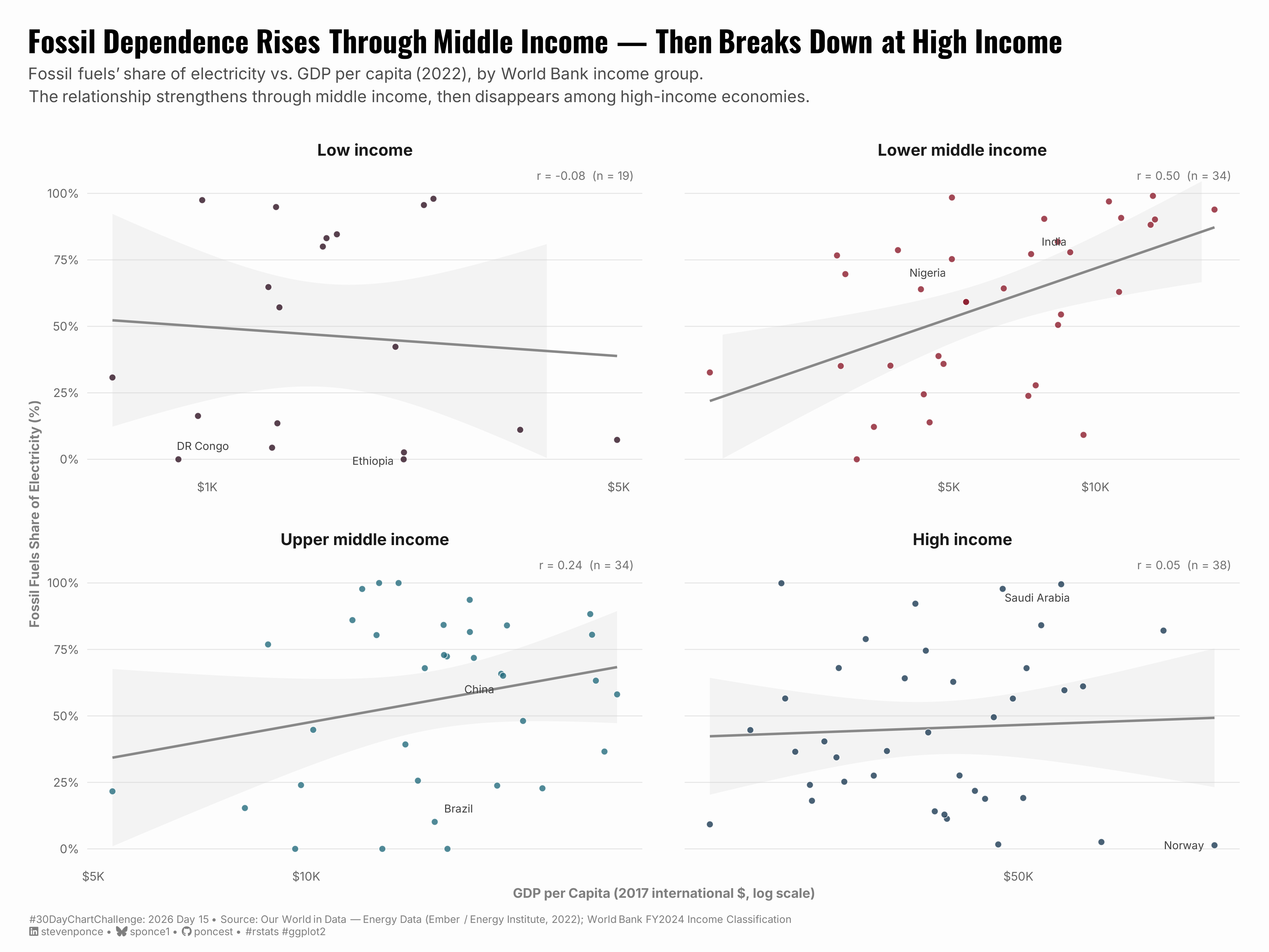
Fossil Dependence Rises Through Middle Income — Then Breaks Down at High Income

Fossil fuels’ share of electricity vs. GDP per capita (2022), by World Bank income group. The relationship strengthens through middle income, then disappears among high-income economies.

A faceted scatter plot exploring how the correlation between fossil fuel dependence and GDP per capita shifts across World Bank income groups. Using OWID energy data for 2022, each panel shows a distinct relationship: the correlation strengthens through lower- and upper-middle-income economies, then effectively disappears among high-income countries — revealing that wealth enables the energy transition, but does not guarantee it. Built with ggplot2 in R.

Figure 1: A 2×2 grid of scatter plots showing fossil fuels’ share of electricity versus GDP per capita (log scale) in 2022, faceted by World Bank income group. Each panel includes a linear trend line with confidence band and a Pearson r annotation. Low-income countries show no relationship (r = −0.08); lower-middle-income countries show a moderate positive correlation (r = 0.50); upper-middle-income countries show a weak positive trend (r = 0.24); high-income countries show virtually no relationship (r = 0.05). Selected countries are labeled: DR Congo and Ethiopia (low income), Nigeria and India (lower middle), China and Brazil (upper middle), Saudi Arabia and Norway (high income). The overall pattern reveals that fossil dependence rises with income through the middle-income stages, then breaks down at high income — where energy policy choices, not wealth alone, determine the electricity mix.

Steps to Create this Graphic

1. Load Packages & Setup

```{r}
#| label: load
#| warning: false
#| message: false      
#| results: "hide"     

## 1. LOAD PACKAGES & SETUP ----
suppressPackageStartupMessages({
pacman::p_load(
  tidyverse, ggtext, showtext,  
  janitor, scales, glue, ggrepel
  )
})

### |- figure size ----
camcorder::gg_record(
  dir    = here::here("temp_plots"),
  device = "png",
  width  = 12,
  height = 9,
  units  = "in",
  dpi    = 320
)

# Source utility functions
suppressMessages(source(here::here("R/utils/fonts.R")))
source(here::here("R/utils/social_icons.R"))
source(here::here("R/utils/image_utils.R"))
source(here::here("R/themes/base_theme.R"))
```

2. Read in the Data

```{r}
#| label: read
#| include: true
#| eval: true
#| warning: false

owid_energy <- read_csv(
  here::here("data/30DayChartChallenge/2026/owid-energy-data.csv"),
  locale = locale(encoding = "latin1")
  ) |>
  clean_names() 
```

3. Examine the Data

```{r}
#| label: examine
#| include: true
#| eval: true
#| results: 'hide'
#| warning: false

glimpse(owid_energy)

owid_energy |>
  filter(year == 2022) |>
  select(country, iso_code, gdp, population, fossil_share_elec) |>
  skimr::skim()
```

4. Tidy Data

```{r}
#| label: tidy
#| warning: false

### |- World Bank FY2024 income classification ----
# Sourced from: https://databank.worldbank.org/data/download/site-content/CLASS.xlsx
wb_income <- tribble(
  ~country,                              ~income_group,
  "Afghanistan",                         "Low income",
  "Albania",                             "Upper middle income",
  "Algeria",                             "Lower middle income",
  "Angola",                              "Lower middle income",
  "Argentina",                           "Upper middle income",
  "Armenia",                             "Upper middle income",
  "Australia",                           "High income",
  "Austria",                             "High income",
  "Azerbaijan",                          "Upper middle income",
  "Bangladesh",                          "Lower middle income",
  "Belarus",                             "Upper middle income",
  "Belgium",                             "High income",
  "Benin",                               "Low income",
  "Bolivia",                             "Lower middle income",
  "Bosnia and Herzegovina",              "Upper middle income",
  "Brazil",                              "Upper middle income",
  "Bulgaria",                            "Upper middle income",
  "Burkina Faso",                        "Low income",
  "Burundi",                             "Low income",
  "Cambodia",                            "Lower middle income",
  "Cameroon",                            "Lower middle income",
  "Canada",                              "High income",
  "Chad",                                "Low income",
  "Chile",                               "High income",
  "China",                               "Upper middle income",
  "Colombia",                            "Upper middle income",
  "Congo",                               "Lower middle income",
  "Costa Rica",                          "Upper middle income",
  "Croatia",                             "High income",
  "Czech Republic",                      "High income",
  "Democratic Republic of Congo",        "Low income",
  "Denmark",                             "High income",
  "Dominican Republic",                  "Upper middle income",
  "Ecuador",                             "Upper middle income",
  "Egypt",                               "Lower middle income",
  "El Salvador",                         "Lower middle income",
  "Estonia",                             "High income",
  "Ethiopia",                            "Low income",
  "Finland",                             "High income",
  "France",                              "High income",
  "Georgia",                             "Upper middle income",
  "Germany",                             "High income",
  "Ghana",                               "Lower middle income",
  "Greece",                              "High income",
  "Guatemala",                           "Upper middle income",
  "Honduras",                            "Lower middle income",
  "Hungary",                             "High income",
  "India",                               "Lower middle income",
  "Indonesia",                           "Upper middle income",
  "Iran",                                "Lower middle income",
  "Iraq",                                "Upper middle income",
  "Ireland",                             "High income",
  "Israel",                              "High income",
  "Italy",                               "High income",
  "Ivory Coast",                         "Lower middle income",
  "Japan",                               "High income",
  "Jordan",                              "Upper middle income",
  "Kazakhstan",                          "Upper middle income",
  "Kenya",                               "Lower middle income",
  "Kosovo",                              "Upper middle income",
  "Kuwait",                              "High income",
  "Kyrgyzstan",                          "Lower middle income",
  "Laos",                                "Lower middle income",
  "Latvia",                              "High income",
  "Lebanon",                             "Lower middle income",
  "Libya",                               "Upper middle income",
  "Lithuania",                           "High income",
  "Luxembourg",                          "High income",
  "Madagascar",                          "Low income",
  "Malawi",                              "Low income",
  "Malaysia",                            "Upper middle income",
  "Mali",                                "Low income",
  "Mexico",                              "Upper middle income",
  "Moldova",                             "Lower middle income",
  "Mongolia",                            "Lower middle income",
  "Morocco",                             "Lower middle income",
  "Mozambique",                          "Low income",
  "Myanmar",                             "Lower middle income",
  "Nepal",                               "Lower middle income",
  "Netherlands",                         "High income",
  "New Zealand",                         "High income",
  "Nicaragua",                           "Lower middle income",
  "Niger",                               "Low income",
  "Nigeria",                             "Lower middle income",
  "North Macedonia",                     "Upper middle income",
  "Norway",                              "High income",
  "Pakistan",                            "Lower middle income",
  "Panama",                              "Upper middle income",
  "Paraguay",                            "Upper middle income",
  "Peru",                                "Upper middle income",
  "Philippines",                         "Lower middle income",
  "Poland",                              "High income",
  "Portugal",                            "High income",
  "Romania",                             "Upper middle income",
  "Russia",                              "Upper middle income",
  "Rwanda",                              "Low income",
  "Saudi Arabia",                        "High income",
  "Senegal",                             "Lower middle income",
  "Serbia",                              "Upper middle income",
  "Slovakia",                            "High income",
  "Slovenia",                            "High income",
  "South Africa",                        "Upper middle income",
  "South Korea",                         "High income",
  "Spain",                               "High income",
  "Sri Lanka",                           "Lower middle income",
  "Sudan",                               "Low income",
  "Sweden",                              "High income",
  "Switzerland",                         "High income",
  "Syria",                               "Low income",
  "Taiwan",                              "High income",
  "Tajikistan",                          "Low income",
  "Tanzania",                            "Lower middle income",
  "Thailand",                            "Upper middle income",
  "Togo",                                "Low income",
  "Trinidad and Tobago",                 "High income",
  "Tunisia",                             "Lower middle income",
  "Turkey",                              "Upper middle income",
  "Turkmenistan",                        "Upper middle income",
  "Uganda",                              "Low income",
  "Ukraine",                             "Lower middle income",
  "United Arab Emirates",                "High income",
  "United Kingdom",                      "High income",
  "United States",                       "High income",
  "Uruguay",                             "High income",
  "Uzbekistan",                          "Lower middle income",
  "Venezuela",                           "Upper middle income",
  "Vietnam",                             "Lower middle income",
  "Yemen",                               "Low income",
  "Zambia",                              "Low income",
  "Zimbabwe",                            "Lower middle income"
)

### |- ordered factor for income groups ----
income_levels <- c("Low income", "Lower middle income", "Upper middle income", "High income")

### |- filter, compute, join ----
energy_2022 <- owid_energy |>
  filter(
    year == 2022,
    !is.na(iso_code),           
    !is.na(gdp),
    !is.na(population),
    !is.na(fossil_share_elec),
    population > 1e6            
  ) |>
  mutate(gdp_per_capita = gdp / population) |>
  select(country, iso_code, gdp_per_capita, fossil_share_elec) |>
  left_join(wb_income, by = "country") |>
  filter(!is.na(income_group)) |>
  mutate(
    income_group = factor(income_group, levels = income_levels),
    # 2 labels max per panel — policy-relevant or structurally interesting outliers only
    label_flag = case_when(
      country == "Democratic Republic of Congo" ~ "DR Congo",
      country == "Ethiopia"                     ~ "Ethiopia",
      country == "India"                        ~ "India",
      country == "Nigeria"                      ~ "Nigeria",
      country == "China"                        ~ "China",
      country == "Brazil"                       ~ "Brazil",
      country == "Norway"                       ~ "Norway",
      country == "Saudi Arabia"                 ~ "Saudi Arabia",
      TRUE ~ NA_character_
    )
  )

### |- per-panel correlation labels ----
panel_cors <- energy_2022 |>
  group_by(income_group) |>
  summarise(
    r     = cor(log10(gdp_per_capita), fossil_share_elec, use = "complete.obs"),
    n     = n(),
    label = glue("r = {sprintf('%.2f', r)}  (n = {n})")
  )
```

5. Visualization Parameters

```{r}
#| label: params
#| include: true
#| warning: false

### |- plot aesthetics ----
colors <- get_theme_colors(palette = c(
  "Low income"           = "#2E1122",   
  "Lower middle income"  = "#8B1A2A",   
  "Upper middle income"  = "#246B7D",   
  "High income"          = "#1B3A52"    
))

### |- titles and caption ----
title_text    <- "Fossil Dependence Rises Through Middle Income — Then Breaks Down at High Income"

subtitle_text <- str_glue(
  "Fossil fuels' share of electricity vs. GDP per capita (2022), by World Bank income group.<br>",
  "The relationship strengthens through middle income, then disappears among high-income economies."
)
caption_text <- create_dcc_caption(
  dcc_year    = 2026,
  dcc_day     = 15,
  source_text = "Our World in Data — Energy Data (Ember / Energy Institute, 2022); World Bank FY2024 Income Classification"
)

### |- fonts ----
setup_fonts()
fonts <- get_font_families()

### |- base theme ----
base_theme <- create_base_theme(colors)

weekly_theme <- extend_weekly_theme(
  base_theme,
  theme(
    # strip labels
    strip.text   = element_text(
      family = fonts$text, size = 11, face = "bold",
      margin = margin(b = 6)
    ),
    # axes
    axis.title = element_text(family = fonts$text, size = 9, color = "gray50"),
    axis.text = element_text(family = fonts$text, size = 8, color = "gray40"),
    axis.ticks = element_blank(),
    # grid — horizontal only, very faint
    panel.grid.major.y = element_line(color = "gray90", linewidth = 0.3),
    panel.grid.major.x = element_blank(),
    panel.grid.minor = element_blank(),
    # panel spacing — more breathing room
    panel.spacing.x = unit(2.0, "lines"),
    panel.spacing.y = unit(1.8, "lines"),
    # plot margins
    plot.margin = margin(t = 20, r = 20, b = 10, l = 20)
  )
)

theme_set(weekly_theme)
```

6. Plot

```{r}
#| label: plot
#| warning: false

### |- main plot ----
p <- ggplot(energy_2022, aes(x = gdp_per_capita, y = fossil_share_elec)) +
  
  # Geoms
  geom_smooth(
    method = "lm", formula = y ~ x,
    se = TRUE,
    color = "#888888",
    fill  = "gray80",
    linewidth = 0.8,
    alpha = 0.20
  ) +
  geom_point(
    aes(fill = income_group),
    shape = 21,
    sizw = 2.8,
    color = "white",
    stroke = 0.35,
    alpha = 0.80
  ) +
  geom_text_repel(
    aes(label = label_flag),
    family = fonts$text,
    size = 2.6,
    color = "gray25",
    segment.color = "gray65",
    segment.size = 0.3,
    box.padding = 0.4,
    max.overlaps = 10,
    na.rm = TRUE, 
    seed = 42 
  ) +
  geom_text(
    data = panel_cors,
    aes(label = label),
    x = Inf, y = Inf,
    hjust = 1.1, vjust = 1.6,
    family = fonts$text,
    size = 2.8,
    color = "gray45",
    inherit.aes = FALSE
  ) +
  
  # Facets
  facet_wrap(~ income_group, nrow = 2, scales = "free_x") +
  
  # Scales
  scale_x_log10(
    labels = label_dollar(scale_cut = cut_short_scale()),
    breaks = c(500, 1000, 5000, 10000, 50000, 100000)
  ) +
  scale_y_continuous(
    limits = c(0, 105),
    breaks = c(0, 25, 50, 75, 100),
    labels = label_percent(scale = 1)
  ) +
  scale_fill_manual(
    values = colors$palette[income_levels]
    ) +
  # Labs
  labs(
    title = title_text,
    subtitle = subtitle_text,
    caption = caption_text,
    x = "GDP per Capita (2017 international $, log scale)",
    y = "Fossil Fuels Share of Electricity (%)",
    fill = NULL
  ) +
  
  guides(fill = "none") +
  # Theme
  theme(
    legend.position = "none",
    plot.title = element_textbox_simple(
      family = fonts$title, size = 20, face = "bold",
      margin = margin(b = 6)
    ),
    plot.subtitle = element_textbox_simple(
      family = fonts$text, size = 11, color = "gray30",
      lineheight = 1.4,
      margin = margin(b = 25)
    ),
    plot.caption = element_textbox_simple(
      family = fonts$text, size = 7, color = "gray50",
      margin = margin(t = 10)
    )
  )
```

7. Save

```{r}
#| label: save
#| warning: false

### |-  plot image ----  
save_plot(
  p, 
  type = "30daychartchallenge", 
  year = 2026, 
  day = 15, 
  width = 12, 
  height = 9
  )
```

8. Session Info

TipExpand for Session Info

R version 4.3.1 (2023-06-16 ucrt)
Platform: x86_64-w64-mingw32/x64 (64-bit)
Running under: Windows 11 x64 (build 26100)

Matrix products: default


locale:
[1] LC_COLLATE=English_United States.utf8 
[2] LC_CTYPE=English_United States.utf8   
[3] LC_MONETARY=English_United States.utf8
[4] LC_NUMERIC=C                          
[5] LC_TIME=English_United States.utf8    

time zone: America/New_York
tzcode source: internal

attached base packages:
[1] stats     graphics  grDevices utils     datasets  methods   base     

other attached packages:
 [1] here_1.0.2      ggrepel_0.9.8   glue_1.8.0      scales_1.4.0   
 [5] janitor_2.2.1   showtext_0.9-7  showtextdb_3.0  sysfonts_0.8.9 
 [9] ggtext_0.1.2    lubridate_1.9.5 forcats_1.0.1   stringr_1.6.0  
[13] dplyr_1.2.0     purrr_1.2.1     readr_2.2.0     tidyr_1.3.2    
[17] tibble_3.2.1    ggplot2_4.0.2   tidyverse_2.0.0

loaded via a namespace (and not attached):
 [1] gtable_0.3.6       xfun_0.56          htmlwidgets_1.6.4  lattice_0.21-8    
 [5] tzdb_0.5.0         vctrs_0.7.1        tools_4.3.1        generics_0.1.4    
 [9] curl_7.0.0         parallel_4.3.1     gifski_1.32.0-2    pacman_0.5.1      
[13] pkgconfig_2.0.3    Matrix_1.5-4.1     skimr_2.2.2        RColorBrewer_1.1-3
[17] S7_0.2.0           lifecycle_1.0.5    compiler_4.3.1     farver_2.1.2      
[21] textshaping_1.0.4  repr_1.1.7         codetools_0.2-19   snakecase_0.11.1  
[25] litedown_0.9       htmltools_0.5.9    yaml_2.3.12        pillar_1.11.1     
[29] crayon_1.5.3       camcorder_0.1.0    magick_2.8.6       nlme_3.1-162      
[33] commonmark_2.0.0   tidyselect_1.2.1   digest_0.6.39      stringi_1.8.7     
[37] splines_4.3.1      rsvg_2.6.2         rprojroot_2.1.1    fastmap_1.2.0     
[41] grid_4.3.1         cli_3.6.5          magrittr_2.0.3     base64enc_0.1-6   
[45] withr_3.0.2        bit64_4.6.0-1      timechange_0.4.0   rmarkdown_2.30    
[49] bit_4.6.0          otel_0.2.0         ragg_1.5.0         hms_1.1.4         
[53] evaluate_1.0.5     knitr_1.51         markdown_2.0       mgcv_1.8-42       
[57] rlang_1.1.7        gridtext_0.1.6     Rcpp_1.1.1         xml2_1.5.2        
[61] svglite_2.1.3      rstudioapi_0.18.0  vroom_1.7.0        jsonlite_2.0.0    
[65] R6_2.6.1           systemfonts_1.3.2 

9. GitHub Repository

TipExpand for GitHub Repo

The complete code for this analysis is available in 30dcc_2026_15.qmd.

For the full repository, click here.

10. References

TipExpand for References

1. Data Sources:
   • Ember & Energy Institute. (2024). Energy data [Dataset]. Our World in Data. https://ourworldindata.org/energy
   • Ritchie, H., Rosado, P., & Roser, M. (2024). Energy. Our World in Data. https://ourworldindata.org/energy
   • World Bank. (2024). World Bank country and lending groups — FY2024 income classification [Dataset]. https://datahelpdesk.worldbank.org/knowledgebase/articles/906519

11. Custom Functions Documentation

Note📦 Custom Helper Functions

This analysis uses custom functions from my personal module library for efficiency and consistency across projects.

Functions Used:

• fonts.R: setup_fonts(), get_font_families() - Font management with showtext
• social_icons.R: create_social_caption() - Generates formatted social media captions
• image_utils.R: save_plot() - Consistent plot saving with naming conventions
• base_theme.R: create_base_theme(), extend_weekly_theme(), get_theme_colors() - Custom ggplot2 themes

Why custom functions?
These utilities standardize theming, fonts, and output across all my data visualizations. The core analysis (data tidying and visualization logic) uses only standard tidyverse packages.

Source Code:
View all custom functions → GitHub: R/utils