• Steven Ponce
  • About
  • Data Visualizations
  • Projects
  • Resume
  • Email

On this page

  • Original
  • Makeover
  • Steps to Create this Graphic
    • 1. Load Packages & Setup
    • 2. Read in the Data
    • 3. Examine the Data
    • 4. Tidy Data
    • 5. Visualization Parameters
    • 6. Plot
    • 7. Save
    • 8. Session Info
    • 9. GitHub Repository
    • 10. References
    • 11. Custom Functions Documentation

Older Mario Titles Sold More Copies Than Their Revenue Rank Suggests

  • Show All Code
  • Hide All Code

  • View Source

For each title, revenue rank and units rank are shown — longer gaps mean the two metrics disagree more. Re-releases and budget pricing explain why some classics rank much higher in copies than in dollars.

MakeoverMonday
Data Visualization
R Programming
2026
A dot-and-segment chart redesigning the original Mario Game Sales bar chart. Each title is plotted with two ranked dots — estimated gross revenue and units sold — revealing where the two metrics disagree. Re-releases and budget pricing explain why classics like Yoshi’s Island and All-Stars rank much higher in copies than in dollars.
Author

Steven Ponce

Published

March 9, 2026

Original

The original visualization comes from Mario Game Sales

Original visualization

Makeover

Figure 1: A dot-and-segment chart showing 20 Mario game titles ranked by both estimated gross revenue (steel blue dot) and units sold (burgundy dot). Titles are sorted by revenue rank, from best to worst. For most top titles, the two dots sit close together, indicating the metrics agree. Three titles stand out with long burgundy segments extending to the right: Super Mario All-Stars, Super Mario Galaxy 2, and Super Mario World 2: Yoshi’s Island — all ranked much lower in revenue than their unit sales would suggest. Annotations explain that re-releases and budget pricing drove high unit counts without proportional revenue.

Steps to Create this Graphic

1. Load Packages & Setup

Show code
```{r}
#| label: load
#| warning: false
#| message: false      
#| results: "hide"     

## 1. LOAD PACKAGES & SETUP ----
suppressPackageStartupMessages({
  if (!require("pacman")) install.packages("pacman")
  pacman::p_load(
    tidyverse, ggtext, showtext, scales, 
    glue, janitor, readxl  
)
})

### |- figure size ----
camcorder::gg_record(
  dir    = here::here("temp_plots"),
  device = "png",
  width  = 10,
  height = 10,
  units  = "in",
  dpi    = 320
)

# Source utility functions
suppressMessages(source(here::here("R/utils/fonts.R")))
source(here::here("R/utils/social_icons.R"))
source(here::here("R/utils/image_utils.R"))
source(here::here("R/themes/base_theme.R"))
```

2. Read in the Data

Show code
```{r}
#| label: read
#| include: true
#| eval: true
#| warning: false
#| 

df_raw <- readxl::read_xlsx(
  here::here("data/MakeoverMonday/2026/MM 2026 wk10.xlsx")) |>
  clean_names()
```

3. Examine the Data

Show code
```{r}
#| label: examine
#| include: true
#| eval: true
#| results: 'hide'
#| warning: false

glimpse(df_raw)
skimr::skim_without_charts(df_raw)
```

4. Tidy Data

Show code
```{r}
#| label: tidy
#| warning: false

### |- "All Consoles" aggregate rows only ----
df_all <- df_raw |>
  filter(console == "All Consoles") |>
  filter(!is.na(sales_units), !is.na(gross_est)) |>
  filter(!str_detect(str_to_lower(title), "^total")) |>
  mutate(
    gross_rank = rank(-gross_est, ties.method = "first"),
    units_rank = rank(-sales_units, ties.method = "first"),
    rank_delta = units_rank - gross_rank # positive = unit over-performer
  )

### |- Top 20 by gross rank ----
plot_data <- df_all |>
  slice_min(gross_rank, n = 20) |>
  mutate(
    title = fct_reorder(title, gross_rank, .desc = TRUE),
    seg_type = case_when(
      rank_delta >= 4 ~ "unit_over",
      rank_delta <= -4 ~ "gross_over",
      TRUE ~ "neutral"
    )
  )

### |- Annotation x-anchor ----
annot_x_fixed <- 23

annot_data <- plot_data |>
  filter(title %in% c(
    "Super Mario World 2: Yoshi's Island",
    "Super Mario All-Stars",
    "Super Mario Galaxy 2"
  )) |>
  mutate(
    annot_label = case_when(
      str_detect(title, "Yoshi") ~
        "SNES budget re-release\nboosted unit count\nwithout matching revenue",
      str_detect(title, "All-Stars") ~
        "Compilation sold widely\nbut at lower per-title\nrevenue",
      str_detect(title, "Galaxy 2") ~
        "Strong unit seller\nbut priced at a\npremium — revenue\nclosely matches"
    ),
    seg_xend = annot_x_fixed - 0.2
  )

### |- Highlight strip rows ----
highlight_rows <- plot_data |>
  filter(seg_type == "unit_over") |>
  pull(title)
```

5. Visualization Parameters

Show code
```{r}
#| label: params
#| include: true
#| warning: false

### |- Colors ----
colors <- get_theme_colors(
  palette = list(
    burgundy      = "#6D1A36",
    steel         = "#4A6FA5",
    neutral_dark  = "#2B2B2B",
    neutral_mid   = "#6B6B6B",
    neutral_light = "#E5E5E5",
    segment_neut  = "#C8C8C8",
    highlight_bg  = "#F5EEF1",
    background    = "#FAFAF9"
  )
)

### |- Titles and caption ----
title_text <- "Older Mario Titles Sold More Copies Than Their Revenue Rank Suggests"

subtitle_text <- glue(
  "For each title, the <b style='color:{colors$palette$steel}'>● revenue rank</b> and ",
  "<b style='color:{colors$palette$burgundy}'>● units rank</b> are shown — longer gaps mean ",
  "the two metrics disagree more.<br>",
  "Re-releases and budget pricing explain why some classics rank much higher in copies than in dollars."
)

caption_text <- create_mm_caption(
  mm_year     = 2026,
  mm_week     = 10,
  source_text = "Fandom — Video Game Sales Wiki"
)

### |- fonts ----
setup_fonts()
fonts <- get_font_families()

### |- plot theme ----
base_theme <- create_base_theme(colors)

weekly_theme <- extend_weekly_theme(
  base_theme,
  theme(
    panel.grid.major.x = element_line(color = "gray90", linewidth = 0.3),
    panel.grid.major.y = element_blank(),
    axis.ticks         = element_blank(),
    # axis.text.y handled per-panel (p_left uses selective bold; p_right hides it)
    axis.text.x        = element_text(size = 9,   color = colors$palette$gray_mid),
    axis.title.x = element_text(
      face = "bold", size = rel(0.85),
      margin = margin(t = 10), family = fonts$subtitle,
      color = "gray40"
    ),
    plot.title = element_text(
      size = rel(1.3), family = fonts$title, face = "bold",
      color = colors$title, lineheight = 1.1, hjust = 0,
      margin = margin(t = 5, b = 3)
    ),
    plot.subtitle = element_markdown(
      size = rel(0.8), family = fonts$subtitle, face = "italic",
      color = alpha(colors$subtitle, 0.9), lineheight = 1.1,
      margin = margin(t = 0, b = 8)
    ),
  )
)

theme_set(weekly_theme)
```

6. Plot

Show code
```{r}
#| label: plot
#| warning: false

p <- plot_data |>
  ggplot(aes(y = title)) +
  # Geoms 
  geom_rect(
    data = plot_data |> filter(seg_type == "unit_over") |>
      mutate(ynum = as.integer(title)),
    aes(
      xmin = -Inf, xmax = Inf,
      ymin = ynum - 0.45, ymax = ynum + 0.45
    ),
    fill = colors$palette$highlight_bg,
    inherit.aes = FALSE
  ) +
  geom_segment(
    aes(
      x         = gross_rank,
      xend      = units_rank,
      yend      = title,
      color     = seg_type,
      linewidth = seg_type
    ),
    lineend = "round"
  ) +
  geom_point(
    aes(x = gross_rank),
    color = colors$palette$steel,
    size  = 3.4, shape = 16
  ) +
  geom_point(
    aes(x = units_rank),
    color = colors$palette$burgundy,
    size  = 3.4, shape = 16
  ) +
  geom_segment(
    data = annot_data,
    aes(
      x    = units_rank + 0.2,
      xend = seg_xend,
      y    = title,
      yend = title
    ),
    color       = colors$palette$neutral_mid,
    linewidth   = 0.35,
    linetype    = "dotted",
    inherit.aes = FALSE
  ) +
  geom_text(
    data   = annot_data,
    aes(x = annot_x_fixed, y = title, label = annot_label),
    hjust      = 0,
    vjust      = 0.5,
    size       = 2.75,
    family     = fonts$text,
    color      = colors$palette$neutral_mid,
    lineheight = 1.3,
    inherit.aes = FALSE
  ) +
  # Scales 
  scale_color_manual(
    values = c(
      "unit_over"  = colors$palette$burgundy,
      "gross_over" = colors$palette$steel,
      "neutral"    = colors$palette$segment_neut
    )
  ) +
  scale_linewidth_manual(
    values = c(
      "unit_over"  = 1.5,
      "gross_over" = 1.5,
      "neutral"    = 0.75
    )
  ) +
  scale_x_continuous(
    breaks = seq(2, 20, by = 2),
    # Extra right expansion to accommodate annotation text
    expand = expansion(mult = c(0.04, 0.38))
  ) +
  
  scale_y_discrete(
    expand = expansion(mult = c(0.04, 0.05))
  ) +
  # Labs
  labs(
    title    = title_text,
    subtitle = subtitle_text,
    caption  = caption_text,
    x        = "Rank  (1 = best)",
    y        = NULL
  ) +
  # Theme
  theme(
    plot.title = element_markdown(
      size = rel(1.6),
      family = fonts$title,
      face = "bold",
      color = colors$title,
      lineheight = 1.15,
      margin = margin(t = 0, b = 5)
    ),
    plot.subtitle = element_markdown(
      size = rel(0.85),
      family = 'sans',                     
      face = "italic",
      color = alpha(colors$subtitle, 0.88),
      lineheight = 1.5,
      margin = margin(t = 5, b = 10)
    ),
    plot.caption = element_markdown(
      size = rel(0.55),
      family = fonts$subtitle,
      color = colors$caption,
      hjust = 0,
      lineheight = 1.4,
      margin = margin(t = 20, b = 5)
    ),
    plot.margin = margin(15, 15, 10, 15)
  )
```

7. Save

Show code
```{r}
#| label: save
#| warning: false

### |-  plot image ----  
save_plot(
  plot = p, 
  type = "makeovermonday", 
  year = current_year,
  week = current_week,
  width = 10, 
  height = 10
  )
```

8. Session Info

TipExpand for Session Info
R version 4.3.1 (2023-06-16 ucrt)
Platform: x86_64-w64-mingw32/x64 (64-bit)
Running under: Windows 11 x64 (build 26100)

Matrix products: default


locale:
[1] LC_COLLATE=English_United States.utf8 
[2] LC_CTYPE=English_United States.utf8   
[3] LC_MONETARY=English_United States.utf8
[4] LC_NUMERIC=C                          
[5] LC_TIME=English_United States.utf8    

time zone: America/New_York
tzcode source: internal

attached base packages:
[1] stats     graphics  grDevices utils     datasets  methods   base     

other attached packages:
 [1] here_1.0.2      readxl_1.4.5    janitor_2.2.1   glue_1.8.0     
 [5] scales_1.4.0    showtext_0.9-7  showtextdb_3.0  sysfonts_0.8.9 
 [9] ggtext_0.1.2    lubridate_1.9.5 forcats_1.0.1   stringr_1.6.0  
[13] dplyr_1.2.0     purrr_1.2.1     readr_2.2.0     tidyr_1.3.2    
[17] tibble_3.2.1    ggplot2_4.0.2   tidyverse_2.0.0 pacman_0.5.1   

loaded via a namespace (and not attached):
 [1] gtable_0.3.6       xfun_0.56          htmlwidgets_1.6.4  tzdb_0.5.0        
 [5] vctrs_0.7.1        tools_4.3.1        generics_0.1.4     curl_7.0.0        
 [9] gifski_1.32.0-2    pkgconfig_2.0.3    RColorBrewer_1.1-3 skimr_2.2.2       
[13] S7_0.2.0           lifecycle_1.0.5    compiler_4.3.1     farver_2.1.2      
[17] textshaping_1.0.4  repr_1.1.7         codetools_0.2-19   snakecase_0.11.1  
[21] litedown_0.9       htmltools_0.5.9    yaml_2.3.10        pillar_1.10.2     
[25] camcorder_0.1.0    magick_2.8.6       commonmark_2.0.0   tidyselect_1.2.1  
[29] digest_0.6.37      stringi_1.8.7      rsvg_2.6.2         rprojroot_2.1.1   
[33] fastmap_1.2.0      grid_4.3.1         cli_3.6.4          magrittr_2.0.3    
[37] base64enc_0.1-6    withr_3.0.2        timechange_0.4.0   rmarkdown_2.30    
[41] otel_0.2.0         cellranger_1.1.0   ragg_1.5.0         hms_1.1.4         
[45] evaluate_1.0.5     knitr_1.51         markdown_2.0       rlang_1.1.7       
[49] gridtext_0.1.6     Rcpp_1.1.1         xml2_1.5.2         svglite_2.1.3     
[53] rstudioapi_0.18.0  jsonlite_2.0.0     R6_2.6.1           systemfonts_1.3.2 

9. GitHub Repository

TipExpand for GitHub Repo

The complete code for this analysis is available in mm_2026_10.qmd.

For the full repository, click here.

10. References

TipExpand for References

Primary Data (Makeover Monday): 1. Makeover Monday 2026 Week 10: Mario Game Sales 2. Original Article: Mario — Video Game Sales Wiki - Source: Fandom — Video Game Sales Wiki - Coverage: Estimated lifetime sales (units and gross revenue) for Mario franchise titles across all platforms

Source Data: 3. Dataset: 2026 Week 10 — Mario Game Sales - Source: Fandom Video Game Sales Wiki via data.world/makeovermonday - Data includes: Title, release year, console, estimated units sold, estimated gross revenue - Scope: 47 unique titles across 19 consoles; 87 rows including platform-level breakdowns - Sales figures are estimates and may reflect cumulative lifetime sales through time of publication

Note: All values are reported directly from the source. For this visualization, only “All Consoles” aggregate rows were used (one row per title) to avoid double-counting across platform releases. Gross rank and units rank were derived from the source figures. No external population adjustments or price deflators were applied.

11. Custom Functions Documentation

Note📦 Custom Helper Functions

This analysis uses custom functions from my personal module library for efficiency and consistency across projects.

Functions Used:

  • fonts.R: setup_fonts(), get_font_families() - Font management with showtext
  • social_icons.R: create_social_caption() - Generates formatted social media captions
  • image_utils.R: save_plot() - Consistent plot saving with naming conventions
  • base_theme.R: create_base_theme(), extend_weekly_theme(), get_theme_colors() - Custom ggplot2 themes

Why custom functions?
These utilities standardize theming, fonts, and output across all my data visualizations. The core analysis (data tidying and visualization logic) uses only standard tidyverse packages.

Source Code:
View all custom functions → GitHub: R/utils

Back to top

Citation

BibTeX citation:
@online{ponce2026,
  author = {Ponce, Steven},
  title = {Older {Mario} {Titles} {Sold} {More} {Copies} {Than} {Their}
    {Revenue} {Rank} {Suggests}},
  date = {2026-03-09},
  url = {https://stevenponce.netlify.app/data_visualizations/MakeoverMonday/2026/mm_2026_10.html},
  langid = {en}
}
For attribution, please cite this work as:
Ponce, Steven. 2026. “Older Mario Titles Sold More Copies Than Their Revenue Rank Suggests.” March 9, 2026. https://stevenponce.netlify.app/data_visualizations/MakeoverMonday/2026/mm_2026_10.html.
Source Code
---
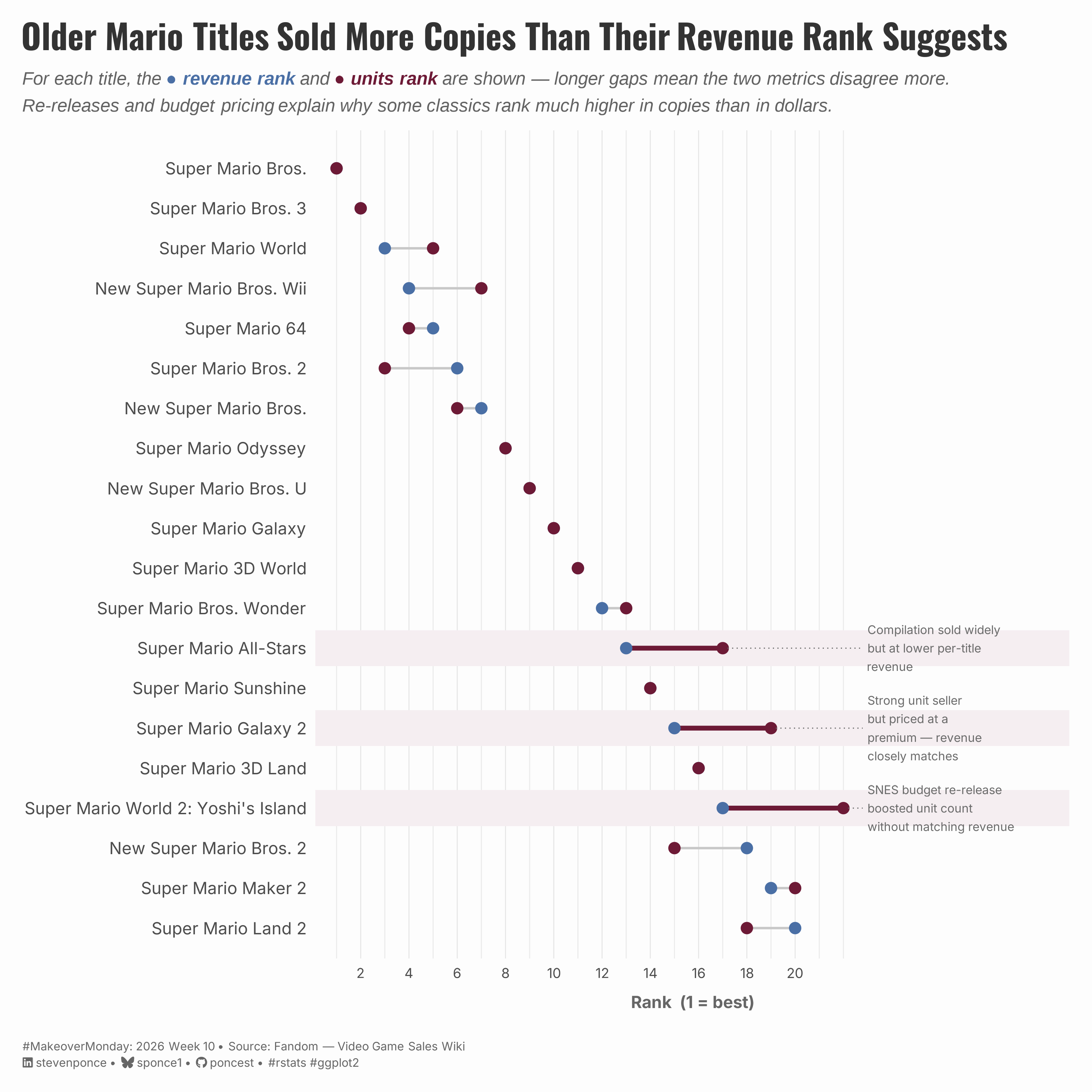
title: "Older Mario Titles Sold More Copies Than Their Revenue Rank Suggests"
subtitle: "For each title, revenue rank and units rank are shown — longer gaps mean the two metrics disagree more. Re-releases and budget pricing explain why some classics rank much higher in copies than in dollars."
description: "A dot-and-segment chart redesigning the original Mario Game Sales bar chart. Each title is plotted with two ranked dots — estimated gross revenue and units sold — revealing where the two metrics disagree. Re-releases and budget pricing explain why classics like Yoshi's Island and All-Stars rank much higher in copies than in dollars."
date: "2026-03-09"
author:
  - name: "Steven Ponce"
    url: "https://stevenponce.netlify.app"
citation:
  url: "https://stevenponce.netlify.app/data_visualizations/MakeoverMonday/2026/mm_2026_10.html"
categories: ["MakeoverMonday", "Data Visualization", "R Programming", "2026"]   
tags: [
  "makeover-monday",
  "dot-plot",
  "ranking",
  "gaming",
  "nintendo",
  "mario",
  "sales-data",
  "ggplot2",
  "patchwork",
  "data-storytelling"
]
image: "thumbnails/mm_2026_10.png"
format:
  html:
    toc: true
    toc-depth: 5
    code-link: true
    code-fold: true
    code-tools: true
    code-summary: "Show code"
    self-contained: true
    theme: 
      light: [flatly, assets/styling/custom_styles.scss]
      dark: [darkly, assets/styling/custom_styles_dark.scss]
editor_options: 
  chunk_output_type: inline
execute: 
  freeze: true                                      
  cache: true                                       
  error: false
  message: false
  warning: false
  eval: true
---

```{r}
#| label: setup-links
#| include: false

# CENTRALIZED LINK MANAGEMENT

## Project-specific info 
current_year <- 2026
current_week <- 10
project_file <- "mm_2026_10.qmd"
project_image <- "mm_2026_10.png"

## Data Sources
data_main <- "https://data.world/makeovermonday/2026w10-mario-game-sales"
data_secondary <- "https://data.world/makeovermonday/2026w10-mario-game-sales"

## Repository Links  
repo_main <- "https://github.com/poncest/personal-website/"
repo_file <- paste0("https://github.com/poncest/personal-website/blob/master/data_visualizations/MakeoverMonday/", current_year, "/", project_file)

## External Resources/Images
chart_original <- "https://raw.githubusercontent.com/poncest/MakeoverMonday/refs/heads/master/2026/Week_10/original_chart.png"

## Organization/Platform Links
org_primary <- "https://vgsales.fandom.com/wiki/Mario#cite_note-vc-27"
org_secondary <- "https://vgsales.fandom.com/wiki/Mario#cite_note-vc-27"

# Helper function to create markdown links
create_link <- function(text, url) {
  paste0("[", text, "](", url, ")")
}

# Helper function for citation-style links
create_citation_link <- function(text, url, title = NULL) {
  if (is.null(title)) {
    paste0("[", text, "](", url, ")")
  } else {
    paste0("[", text, "](", url, ' "', title, '")')
  }
}
```

### Original

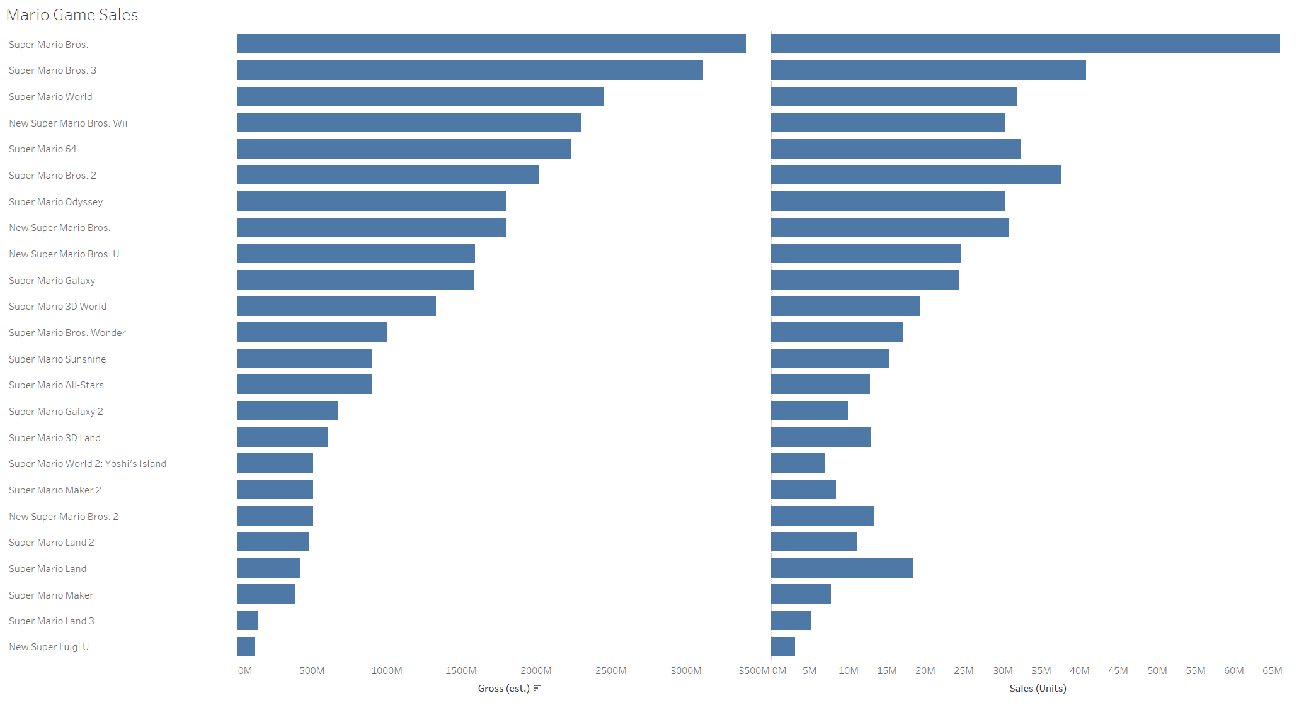
The original visualization comes from `r create_link("Mario Game Sales", data_secondary)`

![Original visualization](https://raw.githubusercontent.com/poncest/MakeoverMonday/refs/heads/master/2026/Week_10/original_chart.png)

### Makeover

![A dot-and-segment chart showing 20 Mario game titles ranked by both estimated gross revenue (steel blue dot) and units sold (burgundy dot). Titles are sorted by revenue rank, from best to worst. For most top titles, the two dots sit close together, indicating the metrics agree. Three titles stand out with long burgundy segments extending to the right: Super Mario All-Stars, Super Mario Galaxy 2, and Super Mario World 2: Yoshi's Island — all ranked much lower in revenue than their unit sales would suggest. Annotations explain that re-releases and budget pricing drove high unit counts without proportional revenue.](mm_2026_10.png){#fig-1}

### [**Steps to Create this Graphic**]{.mark}

#### [1. Load Packages & Setup]{.smallcaps}

```{r}
#| label: load
#| warning: false
#| message: false      
#| results: "hide"     

## 1. LOAD PACKAGES & SETUP ----
suppressPackageStartupMessages({
  if (!require("pacman")) install.packages("pacman")
  pacman::p_load(
    tidyverse, ggtext, showtext, scales, 
    glue, janitor, readxl  
)
})

### |- figure size ----
camcorder::gg_record(
  dir    = here::here("temp_plots"),
  device = "png",
  width  = 10,
  height = 10,
  units  = "in",
  dpi    = 320
)

# Source utility functions
suppressMessages(source(here::here("R/utils/fonts.R")))
source(here::here("R/utils/social_icons.R"))
source(here::here("R/utils/image_utils.R"))
source(here::here("R/themes/base_theme.R"))
```

#### [2. Read in the Data]{.smallcaps}

```{r}
#| label: read
#| include: true
#| eval: true
#| warning: false
#| 

df_raw <- readxl::read_xlsx(
  here::here("data/MakeoverMonday/2026/MM 2026 wk10.xlsx")) |>
  clean_names()
```

#### [3. Examine the Data]{.smallcaps}

```{r}
#| label: examine
#| include: true
#| eval: true
#| results: 'hide'
#| warning: false

glimpse(df_raw)
skimr::skim_without_charts(df_raw)
```

#### [4. Tidy Data]{.smallcaps}

```{r}
#| label: tidy
#| warning: false

### |- "All Consoles" aggregate rows only ----
df_all <- df_raw |>
  filter(console == "All Consoles") |>
  filter(!is.na(sales_units), !is.na(gross_est)) |>
  filter(!str_detect(str_to_lower(title), "^total")) |>
  mutate(
    gross_rank = rank(-gross_est, ties.method = "first"),
    units_rank = rank(-sales_units, ties.method = "first"),
    rank_delta = units_rank - gross_rank # positive = unit over-performer
  )

### |- Top 20 by gross rank ----
plot_data <- df_all |>
  slice_min(gross_rank, n = 20) |>
  mutate(
    title = fct_reorder(title, gross_rank, .desc = TRUE),
    seg_type = case_when(
      rank_delta >= 4 ~ "unit_over",
      rank_delta <= -4 ~ "gross_over",
      TRUE ~ "neutral"
    )
  )

### |- Annotation x-anchor ----
annot_x_fixed <- 23

annot_data <- plot_data |>
  filter(title %in% c(
    "Super Mario World 2: Yoshi's Island",
    "Super Mario All-Stars",
    "Super Mario Galaxy 2"
  )) |>
  mutate(
    annot_label = case_when(
      str_detect(title, "Yoshi") ~
        "SNES budget re-release\nboosted unit count\nwithout matching revenue",
      str_detect(title, "All-Stars") ~
        "Compilation sold widely\nbut at lower per-title\nrevenue",
      str_detect(title, "Galaxy 2") ~
        "Strong unit seller\nbut priced at a\npremium — revenue\nclosely matches"
    ),
    seg_xend = annot_x_fixed - 0.2
  )

### |- Highlight strip rows ----
highlight_rows <- plot_data |>
  filter(seg_type == "unit_over") |>
  pull(title)

```

#### [5. Visualization Parameters]{.smallcaps}

```{r}
#| label: params
#| include: true
#| warning: false

### |- Colors ----
colors <- get_theme_colors(
  palette = list(
    burgundy      = "#6D1A36",
    steel         = "#4A6FA5",
    neutral_dark  = "#2B2B2B",
    neutral_mid   = "#6B6B6B",
    neutral_light = "#E5E5E5",
    segment_neut  = "#C8C8C8",
    highlight_bg  = "#F5EEF1",
    background    = "#FAFAF9"
  )
)

### |- Titles and caption ----
title_text <- "Older Mario Titles Sold More Copies Than Their Revenue Rank Suggests"

subtitle_text <- glue(
  "For each title, the <b style='color:{colors$palette$steel}'>● revenue rank</b> and ",
  "<b style='color:{colors$palette$burgundy}'>● units rank</b> are shown — longer gaps mean ",
  "the two metrics disagree more.<br>",
  "Re-releases and budget pricing explain why some classics rank much higher in copies than in dollars."
)

caption_text <- create_mm_caption(
  mm_year     = 2026,
  mm_week     = 10,
  source_text = "Fandom — Video Game Sales Wiki"
)

### |- fonts ----
setup_fonts()
fonts <- get_font_families()

### |- plot theme ----
base_theme <- create_base_theme(colors)

weekly_theme <- extend_weekly_theme(
  base_theme,
  theme(
    panel.grid.major.x = element_line(color = "gray90", linewidth = 0.3),
    panel.grid.major.y = element_blank(),
    axis.ticks         = element_blank(),
    # axis.text.y handled per-panel (p_left uses selective bold; p_right hides it)
    axis.text.x        = element_text(size = 9,   color = colors$palette$gray_mid),
    axis.title.x = element_text(
      face = "bold", size = rel(0.85),
      margin = margin(t = 10), family = fonts$subtitle,
      color = "gray40"
    ),
    plot.title = element_text(
      size = rel(1.3), family = fonts$title, face = "bold",
      color = colors$title, lineheight = 1.1, hjust = 0,
      margin = margin(t = 5, b = 3)
    ),
    plot.subtitle = element_markdown(
      size = rel(0.8), family = fonts$subtitle, face = "italic",
      color = alpha(colors$subtitle, 0.9), lineheight = 1.1,
      margin = margin(t = 0, b = 8)
    ),
  )
)

theme_set(weekly_theme)
```

#### [6. Plot]{.smallcaps}

```{r}
#| label: plot
#| warning: false

p <- plot_data |>
  ggplot(aes(y = title)) +
  # Geoms 
  geom_rect(
    data = plot_data |> filter(seg_type == "unit_over") |>
      mutate(ynum = as.integer(title)),
    aes(
      xmin = -Inf, xmax = Inf,
      ymin = ynum - 0.45, ymax = ynum + 0.45
    ),
    fill = colors$palette$highlight_bg,
    inherit.aes = FALSE
  ) +
  geom_segment(
    aes(
      x         = gross_rank,
      xend      = units_rank,
      yend      = title,
      color     = seg_type,
      linewidth = seg_type
    ),
    lineend = "round"
  ) +
  geom_point(
    aes(x = gross_rank),
    color = colors$palette$steel,
    size  = 3.4, shape = 16
  ) +
  geom_point(
    aes(x = units_rank),
    color = colors$palette$burgundy,
    size  = 3.4, shape = 16
  ) +
  geom_segment(
    data = annot_data,
    aes(
      x    = units_rank + 0.2,
      xend = seg_xend,
      y    = title,
      yend = title
    ),
    color       = colors$palette$neutral_mid,
    linewidth   = 0.35,
    linetype    = "dotted",
    inherit.aes = FALSE
  ) +
  geom_text(
    data   = annot_data,
    aes(x = annot_x_fixed, y = title, label = annot_label),
    hjust      = 0,
    vjust      = 0.5,
    size       = 2.75,
    family     = fonts$text,
    color      = colors$palette$neutral_mid,
    lineheight = 1.3,
    inherit.aes = FALSE
  ) +
  # Scales 
  scale_color_manual(
    values = c(
      "unit_over"  = colors$palette$burgundy,
      "gross_over" = colors$palette$steel,
      "neutral"    = colors$palette$segment_neut
    )
  ) +
  scale_linewidth_manual(
    values = c(
      "unit_over"  = 1.5,
      "gross_over" = 1.5,
      "neutral"    = 0.75
    )
  ) +
  scale_x_continuous(
    breaks = seq(2, 20, by = 2),
    # Extra right expansion to accommodate annotation text
    expand = expansion(mult = c(0.04, 0.38))
  ) +
  
  scale_y_discrete(
    expand = expansion(mult = c(0.04, 0.05))
  ) +
  # Labs
  labs(
    title    = title_text,
    subtitle = subtitle_text,
    caption  = caption_text,
    x        = "Rank  (1 = best)",
    y        = NULL
  ) +
  # Theme
  theme(
    plot.title = element_markdown(
      size = rel(1.6),
      family = fonts$title,
      face = "bold",
      color = colors$title,
      lineheight = 1.15,
      margin = margin(t = 0, b = 5)
    ),
    plot.subtitle = element_markdown(
      size = rel(0.85),
      family = 'sans',                     
      face = "italic",
      color = alpha(colors$subtitle, 0.88),
      lineheight = 1.5,
      margin = margin(t = 5, b = 10)
    ),
    plot.caption = element_markdown(
      size = rel(0.55),
      family = fonts$subtitle,
      color = colors$caption,
      hjust = 0,
      lineheight = 1.4,
      margin = margin(t = 20, b = 5)
    ),
    plot.margin = margin(15, 15, 10, 15)
  )

```

#### [7. Save]{.smallcaps}

```{r}
#| label: save
#| warning: false

### |-  plot image ----  
save_plot(
  plot = p, 
  type = "makeovermonday", 
  year = current_year,
  week = current_week,
  width = 10, 
  height = 10
  )
```

#### [8. Session Info]{.smallcaps}

::: {.callout-tip collapse="true"}
##### Expand for Session Info

```{r, echo = FALSE}
#| eval: true
#| warning: false

sessionInfo()
```
:::

#### [9. GitHub Repository]{.smallcaps}

::: {.callout-tip collapse="true"}
##### Expand for GitHub Repo

The complete code for this analysis is available in `r create_link(project_file, repo_file)`.

For the full repository, `r create_link("click here", repo_main)`.
:::

#### [10. References]{.smallcaps}

::: {.callout-tip collapse="true"}
##### Expand for References
**Primary Data (Makeover Monday):**
1.  Makeover Monday `r current_year` Week `r current_week`: `r create_link("Mario Game Sales", data_main)`
2.  Original Article: `r create_link("Mario — Video Game Sales Wiki", "https://vgsales.fandom.com/wiki/Mario")`
    -   Source: Fandom — Video Game Sales Wiki
    -   Coverage: Estimated lifetime sales (units and gross revenue) for Mario franchise titles across all platforms

**Source Data:**
3.  Dataset: `r create_link("2026 Week 10 — Mario Game Sales", "https://data.world/makeovermonday/2026w10-mario-game-sales")`
    -   Source: Fandom Video Game Sales Wiki via data.world/makeovermonday
    -   Data includes: Title, release year, console, estimated units sold, estimated gross revenue
    -   Scope: 47 unique titles across 19 consoles; 87 rows including platform-level breakdowns
    -   Sales figures are estimates and may reflect cumulative lifetime sales through time of publication

**Note:** All values are reported directly from the source. For this visualization, only "All Consoles" aggregate rows were used (one row per title) to avoid double-counting across platform releases. Gross rank and units rank were derived from the source figures. No external population adjustments or price deflators were applied.
:::


#### [11. Custom Functions Documentation]{.smallcaps}

::: {.callout-note collapse="true"}
##### 📦 Custom Helper Functions

This analysis uses custom functions from my personal module library for efficiency and consistency across projects.

**Functions Used:**

-   **`fonts.R`**: `setup_fonts()`, `get_font_families()` - Font management with showtext
-   **`social_icons.R`**: `create_social_caption()` - Generates formatted social media captions
-   **`image_utils.R`**: `save_plot()` - Consistent plot saving with naming conventions
-   **`base_theme.R`**: `create_base_theme()`, `extend_weekly_theme()`, `get_theme_colors()` - Custom ggplot2 themes

**Why custom functions?**\
These utilities standardize theming, fonts, and output across all my data visualizations. The core analysis (data tidying and visualization logic) uses only standard tidyverse packages.

**Source Code:**\
View all custom functions → [GitHub: R/utils](https://github.com/poncest/personal-website/tree/master/R)
:::

© 2024 Steven Ponce

Source Issues