Atlantic Hurricanes: The Late-Century Lull

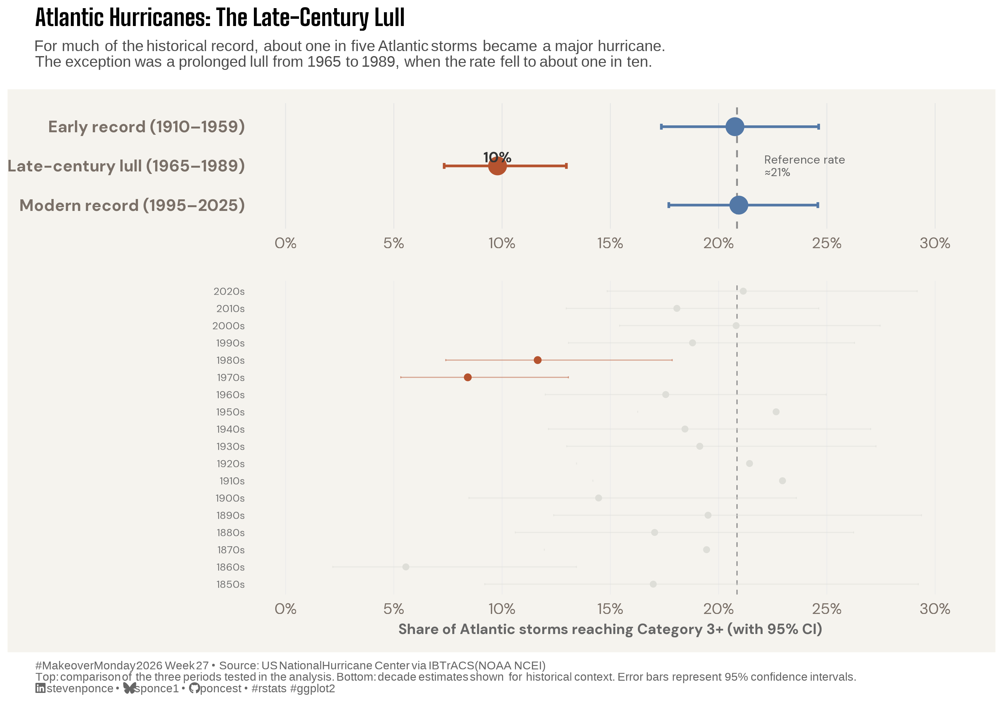
For much of the historical record, about one in five Atlantic storms became a major hurricane. The exception was a prolonged lull from 1965 to 1989, when the rate fell to about one in ten.

A two-panel dot-and-whisker chart comparing the share of Atlantic storms reaching Category 3+ across three historical periods, finding today’s rate is comparable to the early twentieth century while the true statistical outlier was a 1965-1989 lull. Built from IBTrACS storm-level data using binomial confidence intervals and two-proportion tests to validate the periods shown. Created in R with ggplot2, patchwork, and binom.

Original

The original visualization comes from Historical Tropical Cyclones

Original visualization

Makeover

Figure 1: Two-panel dot-and-whisker chart titled “Atlantic Hurricanes: The Late-Century Lull.” The top panel compares the share of Atlantic storms reaching Category 3+ across three tested periods: the early record (1910–1959) at 21%, the late-century lull (1965–1989) at 10%, and the modern record (1995–2025) at 21%, each shown with 95% confidence intervals and a dashed reference line near 21%. The lull, highlighted in red, is the only period whose interval falls clearly below the reference rate. The bottom panel shows the same rate estimated for all 18 decades from the 1850s to the 2020s in muted gray, with the 1970s and 1980s highlighted in red to provide historical context for the top panel’s finding. Data from the US National Hurricane Center via IBTrACS (NOAA NCEI).

Steps to Create this Graphic

1. Load Packages & Setup

```{r}
#| label: load
#| warning: false
#| message: false      
#| results: "hide"     

## 1. LOAD PACKAGES & SETUP ----
suppressPackageStartupMessages({
  if (!require("pacman")) install.packages("pacman")
  pacman::p_load(
    tidyverse, ggtext, showtext, scales, glue, 
  janitor, patchwork, binom, purrr
)
})

### |- figure size ----
camcorder::gg_record(
  dir    = here::here("temp_plots"),
  device = "png",
  width  = 10,
  height = 7,
  units  = "in",
  dpi    = 320
)

# Source utility functions
suppressMessages(source(here::here("R/utils/fonts.R")))
source(here::here("R/utils/social_icons.R"))
source(here::here("R/utils/image_utils.R"))
source(here::here("R/themes/base_theme.R"))
```

2. Read in the Data

```{r}
#| label: read
#| include: true
#| eval: true
#| warning: false
#| 

df_raw <- read_csv(
  here::here("data/MakeoverMonday/2026/ibtracs_lite.csv", na = "")) |>
  clean_names()
```

3. Examine the Data

```{r}
#| label: examine
#| include: true
#| eval: true
#| results: 'hide'
#| warning: false

glimpse(df_raw)
skimr::skim_without_charts(df_raw)
```

4. Tidy Data

```{r}
#| label: tidy
#| warning: false

### |- 4a. Recover blank Atlantic basin field ----
df_raw <- df_raw |>
  mutate(
    basin = case_when(
      !is.na(basin) ~ basin,
      subbasin %in% c("GM", "CS") ~ "NA",
      is.na(subbasin) & lat >= 0 & lat <= 50 &
        lon >= -100 & lon <= 0 ~ "NA",
      TRUE ~ basin
    )
  )

### |- 4b. Collapse to storm level ----
storms <- df_raw |>
  filter(season_year <= 2025) |>
  summarise(
    basin = first(basin[!is.na(basin)]),
    max_sshs = if (all(is.na(usa_sshs))) NA_real_ else max(usa_sshs, na.rm = TRUE),
    max_wind_kts = if (all(is.na(usa_wind_kts))) NA_real_ else max(usa_wind_kts, na.rm = TRUE),
    .by = c(sid, season_year)
  ) |>
  mutate(max_sshs = na_if(max_sshs, -5))

storms_na <- storms |>
  filter(basin == "NA", !is.na(max_sshs)) |>
  mutate(major = as.integer(max_sshs >= 3))

### |- 4c. THE THREE ERAS ---

era_windows <- tribble(
  ~era_label, ~yr_start, ~yr_end, ~era_type,
  "Early record (1910\u20131959)", 1910, 1959, "normal",
  "Late-century lull (1965\u20131989)", 1965, 1989, "trough",
  "Modern record (1995\u20132025)", 1995, 2025, "normal"
)

era_stats <- era_windows |>
  mutate(
    n_total = map2_int(yr_start, yr_end, ~ storms_na |>
      filter(season_year >= .x, season_year <= .y) |>
      nrow()),
    n_major = map2_int(yr_start, yr_end, ~ storms_na |>
      filter(season_year >= .x, season_year <= .y) |>
      pull(major) |>
      sum())
  ) |>
  mutate(
    ci = map2(n_major, n_total, ~ binom.confint(.x, .y, methods = "wilson"))
  ) |>
  unnest(ci) |>
  transmute(era_label, era_type, n_total, n_major,
    pct_major = mean * 100, ci_lower = lower * 100, ci_upper = upper * 100
  )

# Baseline: pooled peak + recent (the two eras confirmed statistically
# indistinguishable, p = 1.0) -- the honest "normal" reference
baseline_data <- storms_na |>
  filter((season_year >= 1910 & season_year <= 1959) |
    (season_year >= 1995 & season_year <= 2025))
baseline <- 100 * mean(baseline_data$major)

### |- 4d. Full decade table ---
decade_stats <- storms_na |>
  mutate(decade = (season_year %/% 10) * 10) |>
  summarise(n_total = n(), n_major = sum(major), .by = decade) |>
  arrange(decade) |>
  mutate(
    ci = map2(n_major, n_total, ~ binom::binom.confint(.x, .y, methods = "wilson"))
  ) |>
  unnest(ci) |>
  select(decade, n_total, n_major, pct_major = mean, ci_lower = lower, ci_upper = upper) |>
  mutate(
    pct_major = pct_major * 100, ci_lower = ci_lower * 100, ci_upper = ci_upper * 100,
    decade_label = paste0(decade, "s"),
    in_trough = decade %in% c(1970, 1980)
  )
```

5. Visualization Parameters

```{r}
#| label: params
#| include: true
#| warning: false

### |- 5a. plot aesthetics ----
colors <- get_theme_colors(
  palette = list(
    trough   = "#B5532F",
    normal   = "#5378A6",
    context  = "#DEDED8",
    baseline = "#8C8C8C"
  )
)
if (is.null(colors$trough)) colors$trough <- "#B5532F"
if (is.null(colors$normal)) colors$normal <- "#5378A6"
if (is.null(colors$context)) colors$context <- "#DEDED8"
if (is.null(colors$baseline)) colors$baseline <- "#8C8C8C"

### |- 5b. titles and caption ----
title_text <- "Atlantic Hurricanes: The Late-Century Lull"

subtitle_text <- str_glue(
  "For much of the historical record, about one in five Atlantic storms became a major ",
  "hurricane.<br>The exception was a prolonged lull from 1965 to 1989, when the rate ",
  "fell to about one in ten."
)

caption_text <- create_mm_caption(
  mm_year = 2026,
  mm_week = 27,
  source_text = paste0(
    "US National Hurricane Center via IBTrACS (NOAA NCEI)<br>",
    "Top: comparison of the three periods tested in the analysis. Bottom: decade ",
    "estimates shown for historical context. Error bars represent 95% confidence intervals."
  )
)

### |- 5c. fonts ----
setup_fonts()
fonts <- get_font_families()

### |- 5d. plot theme ----
base_theme <- create_base_theme(colors)

headline_theme <- extend_weekly_theme(
  base_theme,
  theme(
    plot.title = element_markdown(size = rel(1.3), face = "bold", margin = margin(b = 6)),
    plot.subtitle = element_markdown(size = rel(0.9), color = "gray30", margin = margin(b = 14)),
    panel.grid.major.x = element_line(color = "gray90", linewidth = 0.3),
    panel.grid.major.y = element_blank(),
    panel.grid.minor = element_blank(),
    axis.ticks = element_blank(),
    axis.text.y = element_text(size = rel(1.05), face = "bold"),
    legend.position = "none"
  )
)

context_theme <- extend_weekly_theme(
  base_theme,
  theme(
    panel.grid.major.x = element_line(color = "gray92", linewidth = 0.25),
    panel.grid.major.y = element_blank(),
    panel.grid.minor = element_blank(),
    axis.ticks = element_blank(),
    axis.text.y = element_text(size = rel(0.68), color = "gray45"),
    axis.title.x = element_text(size = rel(0.8), color = "gray40"),
    legend.position = "none"
  )
)
```

6. Plot

```{r}
#| label: plot
#| warning: false

### |- 6a. headline panel ----
p_headline <- era_stats |>
  ggplot(aes(x = pct_major, y = era_label)) +
  geom_vline(
    xintercept = baseline, color = colors$baseline,
    linewidth = 0.6, linetype = "dashed"
  ) +
  annotate(
    "text",
    x = baseline + 1.3, y = "Late-century lull (1965\u20131989)",
    label = paste0("Reference rate\n\u2248", round(baseline), "%"),
    size = 2.9, color = "gray40", family = fonts$text,
    hjust = 0, vjust = 0.5, lineheight = 0.9
  ) +
  geom_errorbar(
    aes(xmin = ci_lower, xmax = ci_upper, color = era_type),
    orientation = "y", width = 0.15, linewidth = 0.9
  ) +
  geom_point(aes(color = era_type), size = 5.5) +
  geom_text(
    data = ~ filter(.x, era_type == "trough"),
    aes(label = paste0(round(pct_major), "%")),
    nudge_y = 0.22, size = 3.6, fontface = "bold", family = fonts$text,
    color = "gray20"
  ) +
  scale_color_manual(values = c(normal = colors$normal, trough = colors$trough)) +
  scale_y_discrete(limits = c(
    "Modern record (1995\u20132025)",
    "Late-century lull (1965\u20131989)",
    "Early record (1910\u20131959)"
  )) +
  scale_x_continuous(
    labels = \(x) paste0(x, "%"), limits = c(0, 30),
    breaks = pretty_breaks(n = 6)
  ) +
  labs(x = NULL, y = NULL) +
  headline_theme

### |- 6b. context panel: full decade record, muted except trough decades ----
p_context <- decade_stats |>
  mutate(decade_label = fct_inorder(decade_label)) |>
  ggplot(aes(x = pct_major, y = decade_label)) +
  geom_vline(
    xintercept = baseline, color = colors$baseline,
    linewidth = 0.4, linetype = "dashed"
  ) +
  geom_errorbar(
    aes(xmin = ci_lower, xmax = ci_upper, color = in_trough),
    orientation = "y", width = 0.12, linewidth = 0.35, alpha = 0.5
  ) +
  geom_point(aes(color = in_trough, size = in_trough)) +
  scale_color_manual(values = c(`TRUE` = colors$trough, `FALSE` = colors$context)) +
  scale_size_manual(values = c(`TRUE` = 1.8, `FALSE` = 1.5), guide = "none") +
  scale_x_continuous(
    labels = \(x) paste0(x, "%"), limits = c(0, 30),
    breaks = pretty_breaks(n = 6)
  ) +
  labs(x = "Share of Atlantic storms reaching Category 3+ (with 95% CI)", y = NULL) +
  context_theme

### |- 6c. combine ----
p_combined <- p_headline / p_context +
  plot_layout(heights = c(1, 2.5)) +
  plot_annotation(
    title = title_text,
    subtitle = subtitle_text,
    caption = caption_text,
    theme = theme(
      plot.title = element_text(size = rel(1.5), face = "bold", margin = margin(b = 6), family = "title_1"),
      plot.subtitle = element_markdown(size = rel(1.0), color = "gray30", margin = margin(b = 14)),
      plot.caption = element_markdown(size = rel(0.75), color = "gray40", hjust = 0)
    )
  )
```

7. Save

```{r}
#| label: save
#| warning: false

### |-  plot image ----  
save_plot_patchwork(
  plot = p_combined, 
  type = "makeovermonday", 
  year = current_year,
  week = current_week,
  width = 10, 
  height = 7
  )
```

8. Session Info

TipExpand for Session Info

R version 4.5.3 (2026-03-11 ucrt)
Platform: x86_64-w64-mingw32/x64
Running under: Windows 11 x64 (build 26100)

Matrix products: default
  LAPACK version 3.12.1

locale:
[1] LC_COLLATE=English_United States.utf8 
[2] LC_CTYPE=English_United States.utf8   
[3] LC_MONETARY=English_United States.utf8
[4] LC_NUMERIC=C                          
[5] LC_TIME=English_United States.utf8    

time zone: America/New_York
tzcode source: internal

attached base packages:
[1] stats     graphics  grDevices utils     datasets  methods   base     

other attached packages:
 [1] here_1.0.2      binom_1.1-1.1   patchwork_1.3.2 janitor_2.2.1  
 [5] glue_1.8.0      scales_1.4.0    showtext_0.9-8  showtextdb_3.0 
 [9] sysfonts_0.8.9  ggtext_0.1.2    lubridate_1.9.5 forcats_1.0.1  
[13] stringr_1.6.0   dplyr_1.2.1     purrr_1.2.2     readr_2.2.0    
[17] tidyr_1.3.2     tibble_3.3.1    ggplot2_4.0.3   tidyverse_2.0.0
[21] pacman_0.5.1   

loaded via a namespace (and not attached):
 [1] gtable_0.3.6       xfun_0.57          htmlwidgets_1.6.4  tzdb_0.5.0        
 [5] yulab.utils_0.2.4  vctrs_0.7.3        tools_4.5.3        generics_0.1.4    
 [9] curl_7.0.0         parallel_4.5.3     gifski_1.32.0-2    pkgconfig_2.0.3   
[13] ggplotify_0.1.3    skimr_2.2.2        RColorBrewer_1.1-3 S7_0.2.1          
[17] lifecycle_1.0.5    compiler_4.5.3     farver_2.1.2       textshaping_1.0.5 
[21] repr_1.1.7         codetools_0.2-20   snakecase_0.11.1   litedown_0.9      
[25] htmltools_0.5.9    yaml_2.3.12        crayon_1.5.3       pillar_1.11.1     
[29] camcorder_0.1.0    magick_2.9.1       commonmark_2.0.0   tidyselect_1.2.1  
[33] digest_0.6.39      stringi_1.8.7      rsvg_2.7.0         rprojroot_2.1.1   
[37] fastmap_1.2.0      grid_4.5.3         cli_3.6.6          magrittr_2.0.5    
[41] base64enc_0.1-6    withr_3.0.2        rappdirs_0.3.4     bit64_4.6.0-1     
[45] timechange_0.4.0   rmarkdown_2.31     bit_4.6.0          otel_0.2.0        
[49] hms_1.1.4          evaluate_1.0.5     knitr_1.51         markdown_2.0      
[53] gridGraphics_0.5-1 rlang_1.2.0        gridtext_0.1.6     Rcpp_1.1.1        
[57] xml2_1.5.2         svglite_2.2.2      rstudioapi_0.18.0  vroom_1.7.1       
[61] jsonlite_2.0.0     R6_2.6.1           fs_2.0.1           systemfonts_1.3.2 

9. GitHub Repository

TipExpand for GitHub Repo

The complete code for this analysis is available in mm_2026_27.qmd.

For the full repository, click here.

10. References

TipExpand for References

Primary Data (Makeover Monday):

1. Makeover Monday 2026 Week 27: Historical Tropical Cyclones
   • CSV: 724,816 rows × 17 columns (sid, season_year, basin, subbasin, name, iso_time, nature, lat, lon, wmo_wind_kts, wmo_pres_mb, wmo_agency, dist2land_km, landfall_km, usa_wind_kts, usa_pres_mb, usa_sshs); one row per 3-hourly storm-track fix, global coverage back to 1842
   • The makeover collapses track-point data to one row per storm, filters to the Atlantic basin only, and restricts to complete seasons (through 2025) — a scope narrowed from the raw data’s global, 1842–2026 span to the subset where historical intensity classification is complete enough to support a rate comparison across eras
   • The source extract’s basin field for Atlantic storms was blank for ~123,000 rows (a source-file defect, not a parsing artifact) and was recovered via subbasin codes and geographic bounding, cross-validated against named storms from known Atlantic naming-list years
2. Original Chart: Major Atlantic hurricanes over past century — BBC News
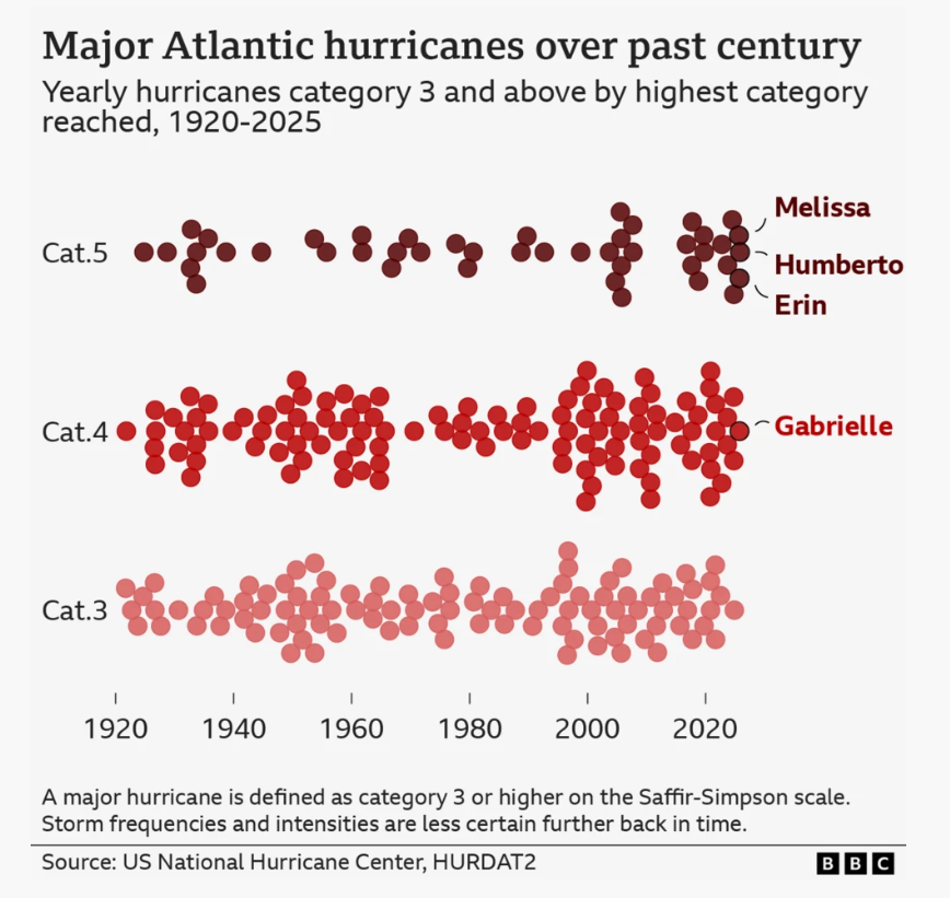
   • A jittered dot plot of raw yearly counts of Category 3+ Atlantic hurricanes, 1920–2025, with select storms (Melissa, Humberto, Erin, Gabrielle) annotated and a general caveat that older records are less certain. The original’s count-based framing implicitly invites the read that today’s activity is elevated — this makeover’s central question tests that implication directly: normalized by total storms tracked and formally compared across eras, does the modern rate of major hurricanes actually stand out, or does the historical record show something else entirely?

Source Data:

3. International Best Track Archive for Climate Stewardship (IBTrACS) — NOAA National Centers for Environmental Information
   • Ultimate source of the storm track records; IBTrACS consolidates tropical cyclone best-track data from multiple international reporting agencies (WMO regional centers and the US National Hurricane Center) into a single global archive, of which this data.world “lite” extract is a track-point-level subset

11. Custom Functions Documentation

Note📦 Custom Helper Functions

This analysis uses custom functions from my personal module library for efficiency and consistency across projects.

Functions Used:

• fonts.R: setup_fonts(), get_font_families() - Font management with showtext
• social_icons.R: create_social_caption() - Generates formatted social media captions
• image_utils.R: save_plot() - Consistent plot saving with naming conventions
• base_theme.R: create_base_theme(), extend_weekly_theme(), get_theme_colors() - Custom ggplot2 themes

Why custom functions?
These utilities standardize theming, fonts, and output across all my data visualizations. The core analysis (data tidying and visualization logic) uses only standard tidyverse packages.

Source Code:
View all custom functions → GitHub: R/utils