Half of Gen Z Investors Have Redirected Investing Dollars to Sports Betting

Redirecting investment funds to sports betting becomes far less common with age

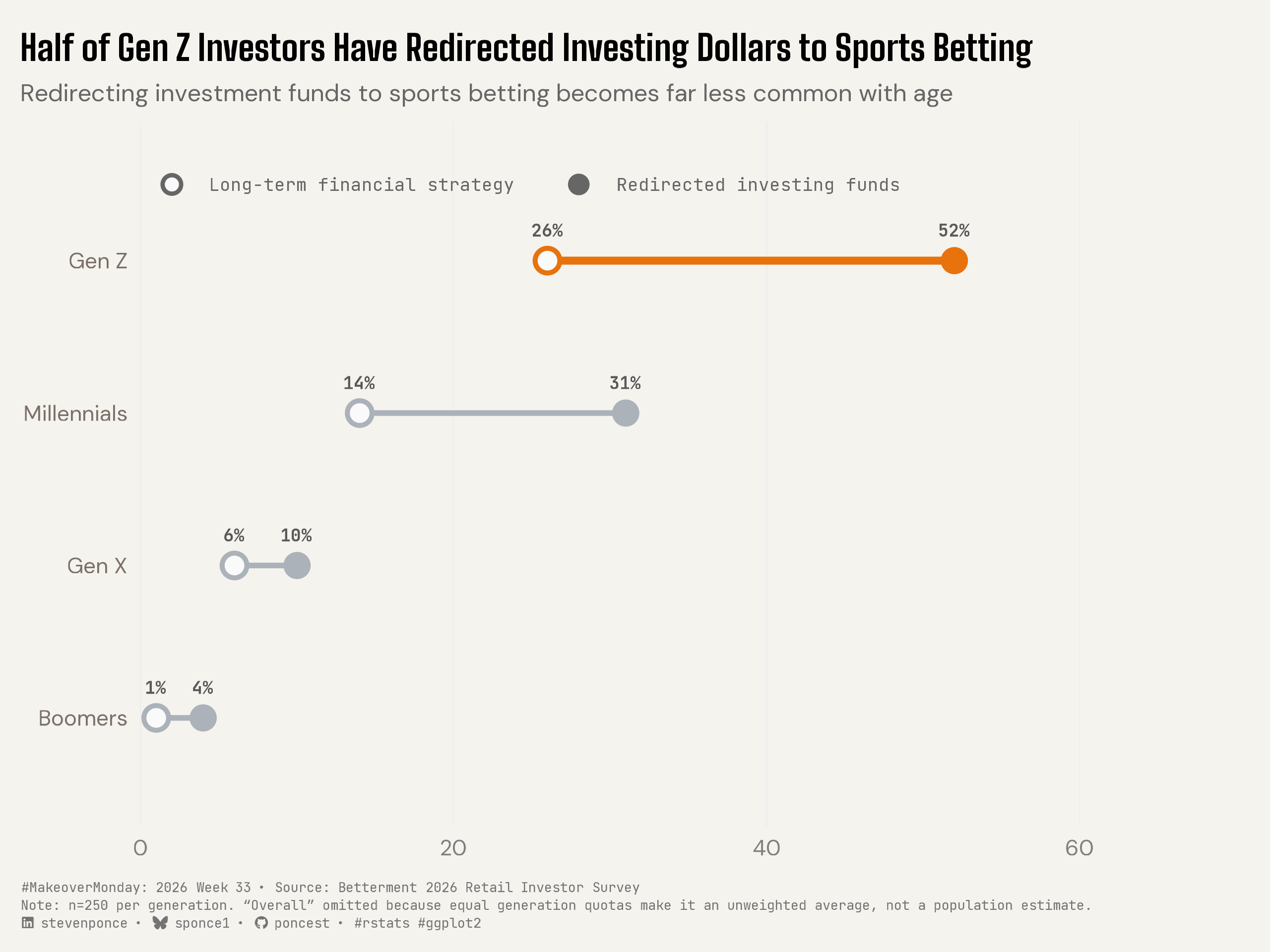
Half of Gen Z investors report redirecting investing funds to sports betting, twice the share who call it part of their long-term financial strategy. A dumbbell chart compares both measures across four generations, using open and filled circles to distinguish the two survey questions. Built in R with ggplot2, ggtext, and ggview.

Original

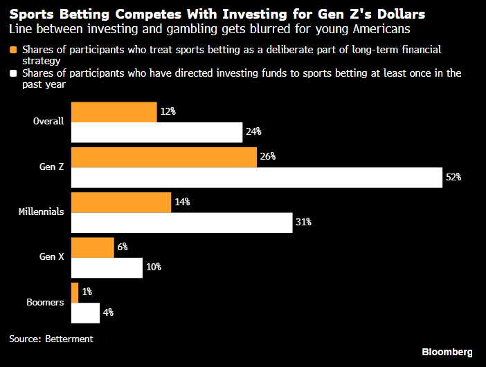
The original visualization comes from Sports Betting in Gen Z Financial Plans

Original visualization

Makeover

Figure 1: Dumbbell chart titled ‘Half of Gen Z Investors Have Redirected Investing Dollars to Sports Betting.’ Each row shows two connected dots per generation: an open circle for the share who consider sports betting part of their long-term financial strategy, and a filled circle for the share who have redirected investing funds to sports betting. Gen Z, highlighted in orange, moves from 26% to 52%. Millennials go from 14% to 31%, Gen X from 6% to 10%, and Boomers from 1% to 4%, showing the gap and the overall share both shrink sharply with age. Source: Betterment 2026 Retail Investor Survey, n=250 per generation.

Steps to Create this Graphic

1. Load Packages & Setup

```{r}
#| label: load
#| warning: false
#| message: false      
#| results: "hide"     

## 1. LOAD PACKAGES & SETUP ----
suppressPackageStartupMessages({
  if (!require("pacman")) install.packages("pacman")
  pacman::p_load(
    tidyverse, ggtext, showtext, scales, glue, janitor, ggview
)
})

# Source utility functions
suppressMessages(
  source(here::here("R/utils/fonts.R")))
  source(here::here("R/utils/social_icons.R"))
  source(here::here("R/themes/base_theme.R"))
```

2. Read in the Data

```{r}
#| label: read
#| include: true
#| eval: true
#| warning: false
#| 

df_raw <- read_csv(
  here::here("data/MakeoverMonday/2026/gen_z_sports_betting_investing.csv"))  |>
  clean_names()
```

3. Examine the Data

```{r}
#| label: examine
#| include: true
#| eval: true
#| results: 'hide'
#| warning: false

glimpse(df_raw)
skimr::skim_without_charts(df_raw)
```

4. Tidy Data

```{r}
#| label: tidy
#| warning: false

df_plot <- df_raw |>
  filter(is_overall == "No") |>
  mutate(
    metric_short = case_when(
      str_detect(metric, regex("deliberate", ignore_case = TRUE)) ~ "deliberate",
      str_detect(metric, regex("redirected|directed", ignore_case = TRUE)) ~ "redirected",
      TRUE ~ metric
    )
  ) |>
  select(generation, metric_short, percent, respondents) |>
  pivot_wider(names_from = metric_short, values_from = percent) |>
  mutate(
    generation = factor(
      generation,
      levels = c("Boomers", "Gen X", "Millennials", "Gen Z")
    ),
    is_hero = generation == "Gen Z",
    gap = redirected - deliberate
  ) |>
  arrange(generation) |>
  mutate(y_pos = as.numeric(generation))
```

5. Visualization Parameters

```{r}
#| label: params
#| include: true
#| warning: false

### |- plot aesthetics ----
colors <- get_theme_colors(
  palette = list(
    hero      = "#E8720C",
    neutral   = "#ABB2B9",
    text_dark = "#1A1A1A"
  )
)
clrs <- colors$palette

### |- titles and caption ----
title_text <- str_glue("Half of Gen Z Investors Have Redirected Investing Dollars to Sports Betting")

subtitle_text <- str_glue("Redirecting investment funds to sports betting becomes far less common with age")

caption_text <- create_mm_caption(
  mm_year = 2026,
  mm_week = 33,
  source_text = "Betterment 2026 Retail Investor Survey<br>Note: n=250 per generation. \"Overall\" omitted because equal generation quotas make it an unweighted average, not a population estimate."
)

### |- fonts ----
setup_fonts()
fonts <- get_font_families()

### |- legend coordinates ----
legend_y <- max(df_plot$y_pos) + 0.5
legend_open_x <- 2
legend_open_label_x <- 4.5
legend_filled_x <- 25
legend_filled_label_x <- 27.5

### |- plot theme ----
base_theme <- create_base_theme(colors)

weekly_theme <- extend_weekly_theme(
  base_theme,
  theme(
    plot.title = element_text(family = fonts$title_1, size = 16, face = "bold"),
    plot.subtitle = element_text(family = fonts$subtitle, size = 11, color = "gray40"),
    plot.caption = element_textbox_simple(
      family = fonts$caption, size = 6, color = "gray45",
      lineheight = 1.35, margin = margin(t = 10)
    ),
    axis.text.y = element_text(family = fonts$body, size = 10),
    axis.text.x = element_text(family = fonts$body, size = 10, color = "gray50"),
    panel.grid.major.y = element_blank(),
    panel.grid.major.x = element_line(color = "gray93", linewidth = 0.25),
    panel.grid.minor = element_blank(),
    axis.ticks = element_blank(),
    legend.position = "none",
    plot.margin = margin(t = 15, r = 20, b = 10, l = 10)
  )
)

theme_set(weekly_theme)
```

6. Plot

```{r}
#| label: plot
#| warning: false

### |- plot ----
p <- ggplot(df_plot) +
  geom_segment(
    aes(
      x = deliberate, xend = redirected, y = y_pos, yend = y_pos,
      color = is_hero, linewidth = is_hero
    ),
    lineend = "round"
  ) +
  geom_point(
    aes(x = deliberate, y = y_pos, color = is_hero),
    shape = 21, fill = "grey98", size = 4.2, stroke = 1.6
  ) +
  geom_point(
    aes(x = redirected, y = y_pos, color = is_hero, fill = is_hero),
    shape = 21, size = 4.2, stroke = 1.2
  ) +
  geom_text(
    aes(x = deliberate, y = y_pos + 0.2, label = paste0(deliberate, "%")),
    family = fonts$caption, size = 2.8, color = "gray35", fontface = "bold"
  ) +
  geom_text(
    aes(x = redirected, y = y_pos + 0.2, label = paste0(redirected, "%")),
    family = fonts$caption, size = 2.8, color = "gray35", fontface = "bold"
  ) +
  annotate(
    "point",
    x = legend_open_x, y = legend_y,
    shape = 21, fill = "grey98", color = "gray40", size = 3, stroke = 1.4
  ) +
  annotate(
    "point",
    x = legend_filled_x + 3, y = legend_y,
    shape = 21, fill = "gray40", color = "gray40", size = 3, stroke = 1.2
  ) +
  geom_text(
    data = tibble(
      x = c(legend_open_label_x, legend_filled_label_x + 3),
      y = c(legend_y, legend_y),
      label = c("Long-term financial strategy", "Redirected investing funds")
    ),
    aes(x = x, y = y, label = label),
    family = fonts$caption, size = 2.85, color = "gray40", hjust = 0,
    inherit.aes = FALSE
  ) +
  scale_color_manual(values = c(`TRUE` = clrs[["hero"]], `FALSE` = clrs[["neutral"]])) +
  scale_fill_manual(values = c(`TRUE` = clrs[["hero"]], `FALSE` = clrs[["neutral"]])) +
  scale_linewidth_manual(values = c(`TRUE` = 1.7, `FALSE` = 1.2)) +
  scale_x_continuous(limits = c(0, 68), expand = expansion(mult = c(0, 0.02))) +
  scale_y_continuous(
    breaks = df_plot$y_pos, labels = df_plot$generation,
    limits = c(min(df_plot$y_pos) - 0.5, max(df_plot$y_pos) + 0.7)
  ) +
  coord_cartesian(clip = "off") +
  labs(
    title = title_text,
    subtitle = subtitle_text,
    caption = caption_text,
    x = NULL, y = NULL
  )
```

7. Save

```{r}
#| label: save
#| warning: false

### |- save ----
main_path  <- here::here("data_visualizations", "MakeoverMonday", "2026", "mm_2026_33.png")
thumb_path <- here::here("data_visualizations", "MakeoverMonday", "2026", "thumbnails", "mm_2026_33.png")

# Full-size version, for the QMD figure
save_ggplot(
  plot = p,
  file = main_path,
  width = 8,
  height = 6,
  units = "in",
  dpi = 320,
  create.dir = TRUE
)

# Reduced-size thumbnail, for the YAML `image:` field
fs::dir_create(dirname(thumb_path))
magick::image_read(main_path) |>
  magick::image_resize("400") |>
  magick::image_write(thumb_path)
```

8. Session Info

TipExpand for Session Info

R version 4.6.1 (2026-06-24)
Platform: aarch64-apple-darwin23
Running under: macOS Tahoe 26.5.2

Matrix products: default
BLAS:   /Library/Frameworks/R.framework/Versions/4.6/Resources/lib/libRblas.0.dylib 
LAPACK: /Library/Frameworks/R.framework/Versions/4.6/Resources/lib/libRlapack.dylib;  LAPACK version 3.12.1

locale:
[1] en_US.UTF-8/en_US.UTF-8/en_US.UTF-8/C/en_US.UTF-8/en_US.UTF-8

time zone: America/New_York
tzcode source: internal

attached base packages:
[1] stats     graphics  grDevices utils     datasets  methods   base     

other attached packages:
 [1] here_1.0.2      ggview_0.2.2    janitor_2.2.1   glue_1.8.1     
 [5] scales_1.4.0    showtext_0.9-8  showtextdb_3.0  sysfonts_0.8.9 
 [9] ggtext_0.1.2    lubridate_1.9.5 forcats_1.0.1   stringr_1.6.0  
[13] dplyr_1.2.1     purrr_1.2.2     readr_2.2.0     tidyr_1.3.2    
[17] tibble_3.3.1    ggplot2_4.0.3   tidyverse_2.0.0 pacman_0.5.1   

loaded via a namespace (and not attached):
 [1] gtable_0.3.6       xfun_0.60          htmlwidgets_1.6.4  tzdb_0.5.0        
 [5] vctrs_0.7.3        tools_4.6.1        generics_0.1.4     curl_7.1.0        
 [9] parallel_4.6.1     pkgconfig_2.0.3    RColorBrewer_1.1-3 skimr_2.2.2       
[13] S7_0.2.2           lifecycle_1.0.5    compiler_4.6.1     farver_2.1.2      
[17] textshaping_1.0.5  repr_1.1.7         codetools_0.2-20   snakecase_0.11.1  
[21] litedown_0.10      htmltools_0.5.9    yaml_2.3.12        pillar_1.11.1     
[25] crayon_1.5.3       magick_2.9.1       commonmark_2.0.0   tidyselect_1.2.1  
[29] digest_0.6.39      stringi_1.8.7      labeling_0.4.3     rprojroot_2.1.1   
[33] fastmap_1.2.0      grid_4.6.1         cli_3.6.6          magrittr_2.0.5    
[37] base64enc_0.1-6    withr_3.0.3        bit64_4.8.2        timechange_0.4.0  
[41] rmarkdown_2.31     bit_4.6.0          otel_0.2.0         ragg_1.5.2        
[45] hms_1.1.4          evaluate_1.0.5     knitr_1.51         markdown_2.0      
[49] rlang_1.3.0        gridtext_0.1.6     Rcpp_1.1.2         xml2_1.6.0        
[53] rstudioapi_0.19.0  vroom_1.7.1        jsonlite_2.0.0     R6_2.6.1          
[57] fs_2.1.0           systemfonts_1.3.2 

9. GitHub Repository

TipExpand for GitHub Repo

The complete code for this analysis is available in mm_2026_33.qmd.

For the full repository, click here.

10. References

TipExpand for References

Primary Data (Makeover Monday):

1. Makeover Monday 2026 Week 33: Sports Betting Competes With Investing for Gen Z’s Dollars
   • CSV: 10 rows × 9 columns (generation, birth_years, metric, percent, respondents, is_overall, survey_field_start, survey_field_end, source). Covers Overall plus four generations (Gen Z, Millennials, Gen X, Boomers), each with two survey measures: share who consider sports betting part of their long-term financial strategy, and share who have redirected investing funds to sports betting at least once. Generation quotas are equal (n=250), so the reported “Overall” row is an unweighted average, not a population estimate.
   • The original visualization presents both measures as paired bars per generation, requiring the reader to subtract to see the gap between what respondents say and what they’ve done. This makeover encodes that gap directly with a dumbbell chart, drops the unweighted “Overall” category, and uses open/filled circles to distinguish the two measures without relying on a color-coded legend for the primary encoding.

Source Data:

2. Betterment, 2026, 2026 Retail Investor Survey

11. Custom Functions Documentation

Note📦 Custom Helper Functions

This analysis uses custom functions from my personal module library for efficiency and consistency across projects.

Functions Used:

• fonts.R: setup_fonts(), get_font_families() - Font management with showtext
• social_icons.R: create_social_caption() - Generates formatted social media captions
• image_utils.R: save_plot() - Consistent plot saving with naming conventions
• base_theme.R: create_base_theme(), extend_weekly_theme(), get_theme_colors() - Custom ggplot2 themes

Why custom functions?
These utilities standardize theming, fonts, and output across all my data visualizations. The core analysis (data tidying and visualization logic) uses only standard tidyverse packages.

Source Code:
View all custom functions → GitHub: R/utils