The deadliest animals rarely kill by attacking us

Estimated annual human deaths by mechanism. Envenomation — mostly snakes — is the surprising middle case: far above direct attacks, well below disease transmission.

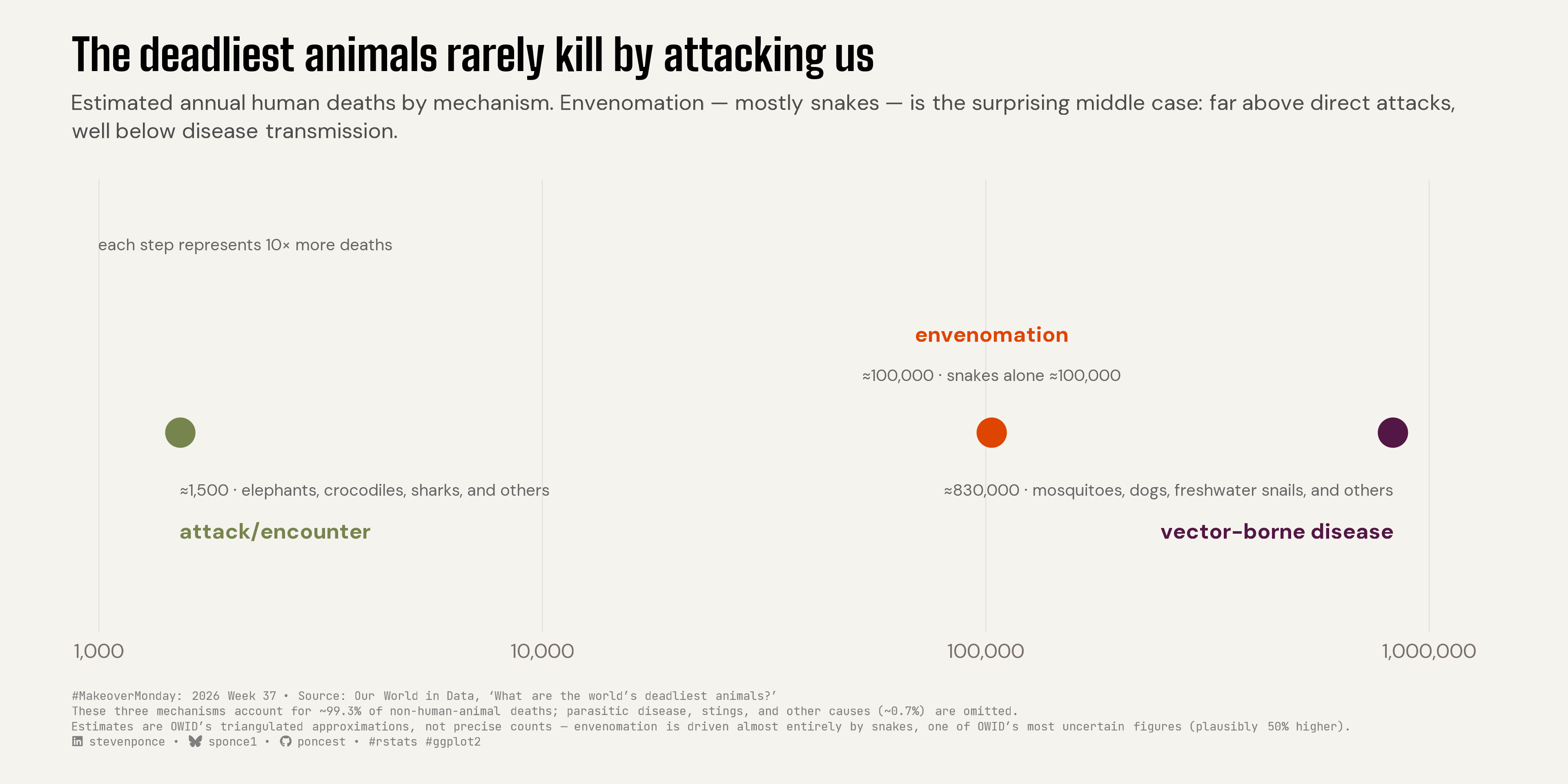
A logarithmic dot plot compares three mechanisms behind an estimated 930,000+ annual animal-caused human deaths: disease transmission (~830,000), envenomation (~100,000, mostly snakes), and direct attack or encounter (~1,500). The redesign reframes Our World in Data’s ranked-by-animal chart around cause of death instead of species, revealing that envenomation sits far closer to disease than to attack. Built in R with ggplot2, ggtext, and showtext.

Original

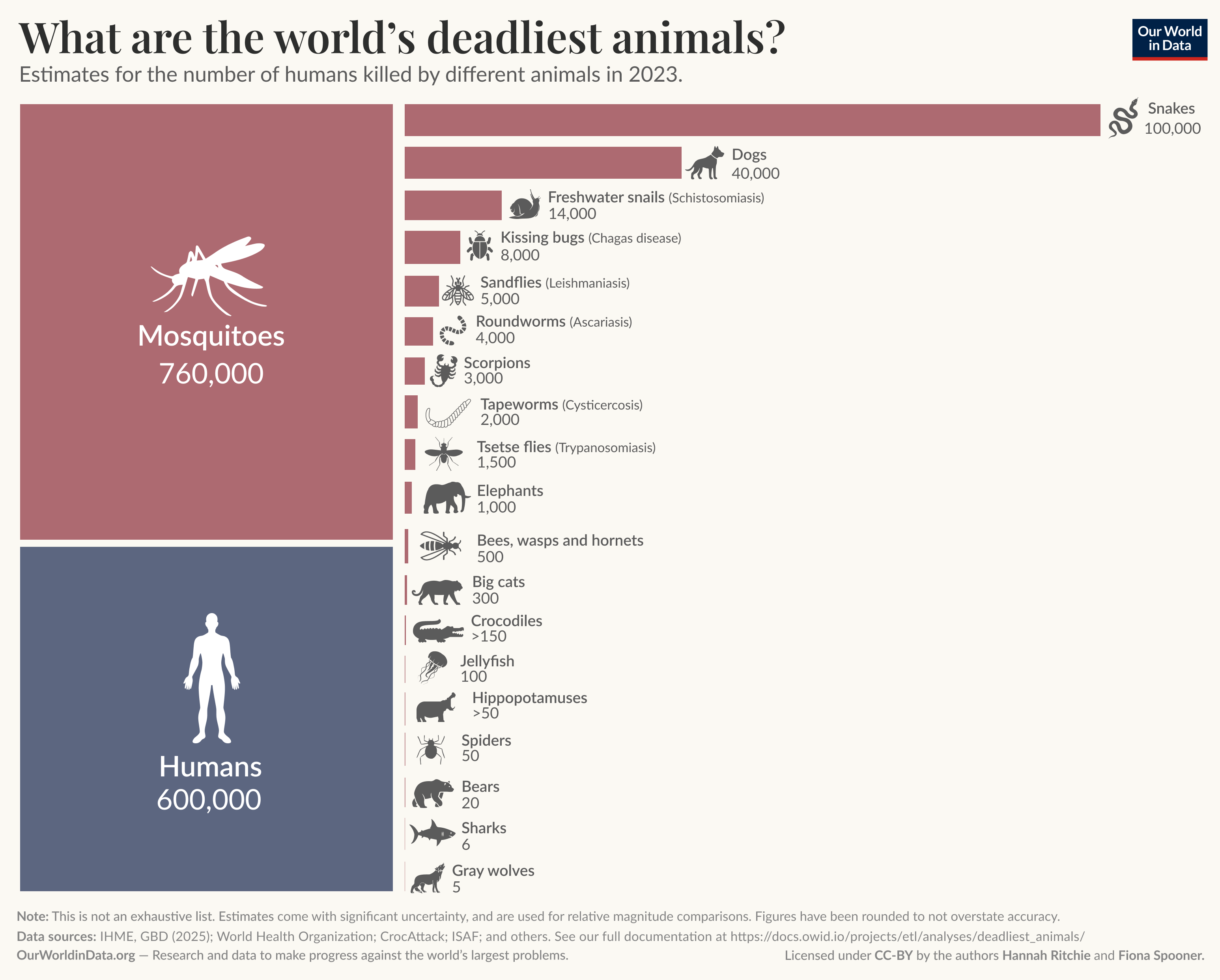
The original visualization comes from What are the world’s deadliest animals?

Original visualization

Makeover

Figure 1: Dot plot on a logarithmic scale comparing three mechanisms behind estimated annual human deaths from animals: attack or encounter, envenomation, and disease transmission, each step representing a tenfold increase. Disease transmission causes an estimated 830,000 deaths, driven mainly by mosquitoes, dogs, and freshwater snails. Envenomation causes about 100,000 deaths, driven almost entirely by snakes. Direct attacks or encounters cause roughly 1,500 deaths. The chart’s key finding is that envenomation, though it might intuitively be grouped with animal attacks, sits far closer in magnitude to disease transmission than to direct attacks. Together, the three mechanisms account for about 99.3 percent of non-human-animal deaths; parasitic disease and stings make up the remaining 0.7 percent. Estimates are Our World in Data’s triangulated approximations and carry meaningful uncertainty, particularly for snakebite-driven envenomation figures. Source: Our World in Data, “What are the world’s deadliest animals?”

Steps to Create this Graphic

1. Load Packages & Setup

```{r}
#| label: load
#| warning: false
#| message: false      
#| results: "hide"     

## 1. LOAD PACKAGES & SETUP ----
suppressPackageStartupMessages({
  if (!require("pacman")) install.packages("pacman")
  pacman::p_load(
    tidyverse, ggtext, showtext, scales, glue, 
  janitor, ggview
)
})

# Source utility functions
suppressMessages(
  source(here::here("R/utils/fonts.R")))
  source(here::here("R/utils/social_icons.R"))
  source(here::here("R/themes/base_theme.R"))
```

2. Read in the Data

```{r}
#| label: read
#| include: true
#| eval: true
#| warning: false
#| 

df_raw <- read_csv(
  here::here("data/MakeoverMonday/2026/worlds_deadliest_animals.csv"))  |>
  clean_names()
```

3. Examine the Data

```{r}
#| label: examine
#| include: true
#| eval: true
#| results: 'hide'
#| warning: false

glimpse(df_raw)
skimr::skim_without_charts(df_raw)
```

4. Tidy Data

```{r}
#| label: tidy
#| warning: false

### |- source-audit enrichment (mechanism classification, derived from
###    OWID's technical documentation text, not from the numbers) ----
df_enriched <- tribble(
  ~animal,               ~deaths, ~mechanism,
  "Mosquitoes",          760000,  "vector-borne disease",
  "Humans",              600000,  "violence/conflict",
  "Snakes",              100000,  "envenomation",
  "Dogs",                40000,   "vector-borne disease",
  "Freshwater snails",   14000,   "vector-borne disease",
  "Kissing bugs",        8000,    "vector-borne disease",
  "Sandflies",           5000,    "vector-borne disease",
  "Roundworms",          4000,    "parasitic disease",
  "Scorpions",           3000,    "envenomation",
  "Tapeworms",           2000,    "parasitic disease",
  "Tsetse flies",        1500,    "vector-borne disease",
  "Elephants",           1000,    "attack/encounter",
  "Bees, wasps, hornets", 500,    "sting/anaphylaxis",
  "Big cats",            300,     "attack/encounter",
  "Crocodiles",          150,     "attack/encounter",
  "Jellyfish",           100,     "envenomation",
  "Hippopotamuses",      50,      "attack/encounter",
  "Spiders",             50,      "envenomation",
  "Bears",               20,      "attack/encounter",
  "Sharks",              6,       "attack/encounter",
  "Gray wolves",         5,       "attack/rabies (mixed)"
)

### |- three-mechanism hero structure  ----
### Covers ~99.3% of the non-human total. Parasitic disease, sting/
### anaphylaxis, and the mixed wolf category (~0.7% combined) are
### disclosed in the caption, not shown as a fourth point.
mechanism_levels <- c("attack/encounter", "envenomation", "vector-borne disease")

total_nonhuman <- df_enriched |>
  filter(animal != "Humans") |>
  summarise(total = sum(deaths)) |>
  pull(total)

df_hero <- df_enriched |>
  filter(animal != "Humans", mechanism %in% mechanism_levels) |>
  summarise(deaths = sum(deaths), .by = mechanism) |>
  mutate(
    mechanism = factor(mechanism, levels = mechanism_levels),
    label_top = mechanism %in% c("envenomation"),
    label_hjust = case_when(
      mechanism == "attack/encounter" ~ 0,
      mechanism == "vector-borne disease" ~ 1,
      TRUE ~ 0.5
    ),
    # round to ~2 significant figures, matching OWID's own stated rounding convention
    deaths_rounded = signif(deaths, 2),
    detail = case_when(
      mechanism == "attack/encounter" ~ "elephants, crocodiles, sharks, and others",
      mechanism == "envenomation" ~ "snakes alone ≈100,000",
      mechanism == "vector-borne disease" ~ "mosquitoes, dogs, freshwater snails, and others"
    )
  )

# display label distinct from the analytical `mechanism` field
df_hero <- df_hero |>
  mutate(
    display_label = case_when(
      mechanism == "vector-borne disease" ~ "disease transmission",
      TRUE ~ as.character(mechanism)
    )
  )

pct_covered <- sum(df_hero$deaths) / total_nonhuman
pct_excluded <- 1 - pct_covered
```

5. Visualization Parameters

```{r}
#| label: params
#| include: true
#| warning: false

### |- plot aesthetics ----
colors <- get_theme_colors(
  palette = list(
    attack = "#76844E", venom = "#DE4500", disease = "#531745"
  )
)

mechanism_colors <- c(
  "attack/encounter"     = colors$palette$attack,
  "envenomation"          = colors$palette$venom,
  "vector-borne disease" = colors$palette$disease
)

### |- titles and caption ----
title_text <- str_glue("The deadliest animals rarely kill by attacking us")

subtitle_text <- str_glue(
  "Estimated annual human deaths by mechanism. Envenomation — mostly ",
  "snakes — is the surprising middle case: far above direct attacks, ",
  "well below disease transmission."
)

caption_text <- create_mm_caption(
  mm_year = 2026,
  mm_week = 37,
  source_text = glue(
    "Our World in Data, 'What are the world's deadliest animals?'<br>",
    "These three mechanisms account for ~{label_percent(accuracy = 0.1)(pct_covered)} ",
    "of non-human-animal deaths; parasitic disease, stings, and other causes ",
    "(~{label_percent(accuracy = 0.1)(pct_excluded)}) are omitted.<br>",
    "Estimates are OWID's triangulated approximations, not precise counts — ",
    "envenomation is driven almost entirely by snakes, one of OWID's most ",
    "uncertain figures (plausibly 50% higher)."
  )
)

### |- fonts ----
setup_fonts()
fonts <- get_font_families()

### |- plot theme ----
base_theme <- create_base_theme(colors)

weekly_theme <- extend_weekly_theme(
  base_theme,
  theme(
    axis.text.y      = element_blank(),
    axis.title       = element_blank(),
    axis.ticks.y      = element_blank(),
    panel.grid.major.y = element_blank(),
    panel.grid.minor   = element_blank(),
    panel.grid.major.x = element_line(color = "gray88", linewidth = 0.25),
    legend.position    = "none",
    plot.margin        = margin(20, 40, 20, 40),
    plot.title.position = "plot",
    plot.title = element_textbox_simple(
      size = 24, face = "bold", family = fonts$title_1,
      width = grid::unit(1, "npc"), lineheight = 1.05,
      margin = margin(b = 10)
    ),
    plot.subtitle = element_textbox_simple(
      size = 12.5, family = fonts$subtitle, color = "grey30",
      width = grid::unit(1, "npc"), margin = margin(t = 2, b = 22)
    ),
    plot.caption = element_textbox_simple(
      size = 8, family = fonts$caption, color = "grey45",
      margin = margin(t = 14)
    ),
  )
)

theme_set(weekly_theme)
```

6. Plot

```{r}
#| label: plot
#| warning: false

### |- plot ----
p <- df_hero |>
  ggplot(aes(x = deaths, y = 0, color = mechanism)) +
  geom_segment(
    x = 1000, xend = 1000000, y = 0, yend = 0,
    color = "gray70", linewidth = 0.4, inherit.aes = FALSE
  ) +
  geom_point(size = 7) +
  geom_text(
    aes(
      label = mechanism,
      y = if_else(label_top, 0.55, -0.55),
      hjust = label_hjust
    ),
    fontface = "bold", size = 4.2, family = fonts$text, show.legend = FALSE
  ) +
  geom_text(
    aes(
      label = glue("≈{comma(deaths_rounded)} · {detail}"),
      y = if_else(label_top, 0.32, -0.32),
      hjust = label_hjust
    ),
    size = 3.2, color = "gray40", family = fonts$text, show.legend = FALSE
  ) +
  annotate(
    "text",
    x = 1000, y = 1.05, hjust = 0, size = 3.2, color = "gray40",
    label = "each step represents 10× more deaths", family = fonts$text
  ) +
  scale_x_log10(
    breaks = c(1e3, 1e4, 1e5, 1e6),
    labels = comma_format(),
    limits = c(1000, 1000000),
    expand = expansion(mult = c(0.02, 0.05))
  ) +
  scale_color_manual(values = mechanism_colors) +
  coord_cartesian(ylim = c(-1, 1.3), clip = "off") +
  labs(
    title = title_text,
    subtitle = subtitle_text,
    caption = caption_text
  ) +
  theme(
    plot.title = element_textbox_simple(
      size = 24, face = "bold", family = fonts$title,
      margin = margin(b = 8)
    ),
    plot.subtitle = element_textbox_simple(
      size = 12, color = "gray30", family = fonts$body,
      margin = margin(b = 20), lineheight = 1.3
    ),
    plot.caption = element_textbox_simple(
      size = 6.5, color = "gray50", family = fonts$body,
      margin = margin(t = 16), lineheight = 1.3
    )
  )
```

7. Save

```{r}
#| label: save
#| warning: false

### |- save ----
main_path  <- here::here("data_visualizations", "MakeoverMonday", "2026", "mm_2026_37.png")
thumb_path <- here::here("data_visualizations", "MakeoverMonday", "2026", "thumbnails", "mm_2026_37.png")

# Full-size version, for the QMD figure
save_ggplot(
  plot = p,
  file = main_path,
  width = 12,
  height = 6,
  units = "in",
  dpi = 320,
  create.dir = TRUE
)

# Reduced-size thumbnail, for the YAML `image:` field
fs::dir_create(dirname(thumb_path))
magick::image_read(main_path) |>
  magick::image_resize("400") |>
  magick::image_write(thumb_path)
```

8. Session Info

TipExpand for Session Info

R version 4.6.1 (2026-06-24)
Platform: aarch64-apple-darwin23
Running under: macOS Tahoe 26.6.2

Matrix products: default
BLAS:   /Library/Frameworks/R.framework/Versions/4.6/Resources/lib/libRblas.0.dylib 
LAPACK: /Library/Frameworks/R.framework/Versions/4.6/Resources/lib/libRlapack.dylib;  LAPACK version 3.12.1

locale:
[1] en_US.UTF-8/en_US.UTF-8/en_US.UTF-8/C/en_US.UTF-8/en_US.UTF-8

time zone: America/New_York
tzcode source: internal

attached base packages:
[1] stats     graphics  grDevices utils     datasets  methods   base     

other attached packages:
 [1] here_1.0.2      ggview_0.2.2    janitor_2.2.1   glue_1.8.1     
 [5] scales_1.4.0    showtext_0.9-8  showtextdb_3.0  sysfonts_0.8.9 
 [9] ggtext_0.1.2    lubridate_1.9.5 forcats_1.0.1   stringr_1.6.0  
[13] dplyr_1.2.1     purrr_1.2.2     readr_2.2.0     tidyr_1.3.2    
[17] tibble_3.3.1    ggplot2_4.0.3   tidyverse_2.0.0 pacman_0.5.1   

loaded via a namespace (and not attached):
 [1] gtable_0.3.6       xfun_0.60          htmlwidgets_1.6.4  tzdb_0.5.0        
 [5] vctrs_0.7.3        tools_4.6.1        generics_0.1.4     curl_7.1.0        
 [9] parallel_4.6.1     pkgconfig_2.0.3    RColorBrewer_1.1-3 skimr_2.2.2       
[13] S7_0.2.2           lifecycle_1.0.5    compiler_4.6.1     farver_2.1.2      
[17] textshaping_1.0.5  repr_1.1.7         codetools_0.2-20   snakecase_0.11.1  
[21] litedown_0.10      htmltools_0.5.9    yaml_2.3.12        pillar_1.11.1     
[25] crayon_1.5.3       magick_2.9.1       commonmark_2.0.0   tidyselect_1.2.1  
[29] digest_0.6.39      stringi_1.8.7      labeling_0.4.3     rprojroot_2.1.1   
[33] fastmap_1.2.0      grid_4.6.1         cli_3.6.6          magrittr_2.0.5    
[37] base64enc_0.1-6    withr_3.0.3        bit64_4.8.2        timechange_0.4.0  
[41] rmarkdown_2.31     bit_4.6.0          otel_0.2.0         ragg_1.5.2        
[45] hms_1.1.4          evaluate_1.0.5     knitr_1.51         markdown_2.0      
[49] rlang_1.3.0        gridtext_0.1.6     Rcpp_1.1.2         xml2_1.6.0        
[53] rstudioapi_0.19.0  vroom_1.7.1        jsonlite_2.0.0     R6_2.6.1          
[57] fs_2.1.0           systemfonts_1.3.2 

9. GitHub Repository

TipExpand for GitHub Repo

The complete code for this analysis is available in mm_2026_37.qmd.

For the full repository, click here.

10. References

TipExpand for References

Primary Data (Makeover Monday): 1. Makeover Monday 2026 Week 37: What are the world’s deadliest animals? - CSV: 21 rows × 4 columns (animal, animal_type, number_of_humans_killed_per_year, estimate_qualifier). Annual estimated human deaths attributed to 20 animal-related causes plus Humans as a reference category, triangulated by Our World in Data from multiple sources (IHME Global Burden of Disease, WHO Global Health Estimates, and peer-reviewed/gray literature) rather than measured directly. estimate_qualifier is populated for only 2 of 21 rows (Crocodiles “>150”, Hippopotamuses “>50”), which understates the dataset’s actual uncertainty — OWID’s own technical documentation states a comparable lower-bound caveat for Bees/wasps/hornets (“more than 500”) that was not carried into the qualifier column, and flags several other estimates (Snakes, Dogs, Elephants) as among its least certain despite carrying no qualifier at all. - The original visualization ranks all 21 causes by raw death count in a single bar chart, dominated visually by Mosquitoes (760,000) with a rapidly compressing tail. This makeover reclassifies the 20 non-human causes by underlying mechanism — vector-borne/disease transmission, envenomation, parasitic disease, direct attack/encounter, sting/anaphylaxis, and one mixed case — derived from OWID’s technical documentation text rather than inferred from the numbers. Humans (600,000) is reported by OWID as a separate reference category (deaths from interpersonal violence and conflict, not animal-caused) and is excluded from the mechanism analysis. The result: three mechanisms account for ~99.3% of non-human-animal deaths, and disease transmission (~830,000) so overwhelms direct attack/encounter (~1,500, a ~550-fold difference) that the intuitive “dangerous animal” framing collapses — with envenomation (~100,000, almost entirely snakes) surfacing as a genuinely surprising middle case, sitting far closer in magnitude to disease transmission than to direct attack.

Source Data: 2. Our World in Data, 2026, What are the world’s deadliest animals? 3. Ritchie, H. & Spooner, F., 2026, Technical documentation and methodology 4. Dataset (CSV): worlds_deadliest_animals.csv

11. Custom Functions Documentation

Note📦 Custom Helper Functions

This analysis uses custom functions from my personal module library for efficiency and consistency across projects.

Functions Used:

• fonts.R: setup_fonts(), get_font_families() - Font management with showtext
• social_icons.R: create_social_caption() - Generates formatted social media captions
• image_utils.R: save_plot() - Consistent plot saving with naming conventions
• base_theme.R: create_base_theme(), extend_weekly_theme(), get_theme_colors() - Custom ggplot2 themes

Why custom functions?
These utilities standardize theming, fonts, and output across all my data visualizations. The core analysis (data tidying and visualization logic) uses only standard tidyverse packages.

Source Code:
View all custom functions → GitHub: R/utils