Tracking Eurovision Wins by Country from 1956 to 2024
SWDchallenge
Data Visualization
R Programming
2024
Author
Steven Ponce
Published
November 1, 2024
Original
The goal of this month’s #SWDchallenge is to make a good graph. For my submission, I decided to revisit a #dataviz from early in my journey. The chart below was my submission for the 2022 #TidyTuesday week 20 challenge. The goal back then was to visualize the countries with more than three Eurovision wins.
Figure 1: Original chart
Additional information about this month’s #SWDchallenge can be found HERE
Makeover
Figure 2: Line chart showing cumulative Eurovision wins by country from 1956 to 2024. Sweden and Ireland lead with 7 wins each, with Ireland’s most recent win in 1996 and Sweden’s in 2023. Other countries have fewer wins, depicted in gray.
Steps to Create this Graphic
1. Load Packages & Setup
Code
```{r}#| label: loadif (!require("pacman")) install.packages("pacman")pacman::p_load( tidyverse, # Easily Install and Load the 'Tidyverse' ggtext, # Improved Text Rendering Support for 'ggplot2' showtext, # Using Fonts More Easily in R Graphs janitor, # Simple Tools for Examining and Cleaning Dirty Data skimr, # Compact and Flexible Summaries of Data scales, # Scale Functions for Visualization glue, # Interpreted String Literals here, # A Simpler Way to Find Your Files tidytuesdayR, # Access the Weekly 'TidyTuesday' Project Dataset ggrepel # Automatically Position Non-Overlapping Text Labels with 'ggplot2') ### |- figure size ---- camcorder::gg_record( dir = here::here("temp_plots"), device ="png",width =10,height =8,units ="in",dpi =320)### |- resolution ---- showtext_opts(dpi =320, regular.wt =300, bold.wt =800)```
---title: "Eurovision: Sweden and Ireland Lead with the Most Wins"subtitle: "Tracking Eurovision Wins by Country from 1956 to 2024"author: "Steven Ponce"date: "2024-11-01"categories: ["SWDchallenge", "Data Visualization", "R Programming", "2024"]image: "thumbnails/swd_2024_11.png"format: html: toc: true toc-depth: 5 code-link: true code-fold: true code-tools: trueeditor_options: chunk_output_type: consoleexecute: error: false message: false warning: false eval: false# share:# permalink: "https://stevenponce.netlify.app/data_visualizations.html"# linkedin: true# twitter: true# email: true---### OriginalThe goal of this month's #SWDchallenge is to _make a good graph_. For my submission, I decided to revisit a #dataviz from early in my journey. The chart below was my submission for the 2022 #TidyTuesday week 20 challenge. The goal back then was to visualize the countries with more than three Eurovision wins.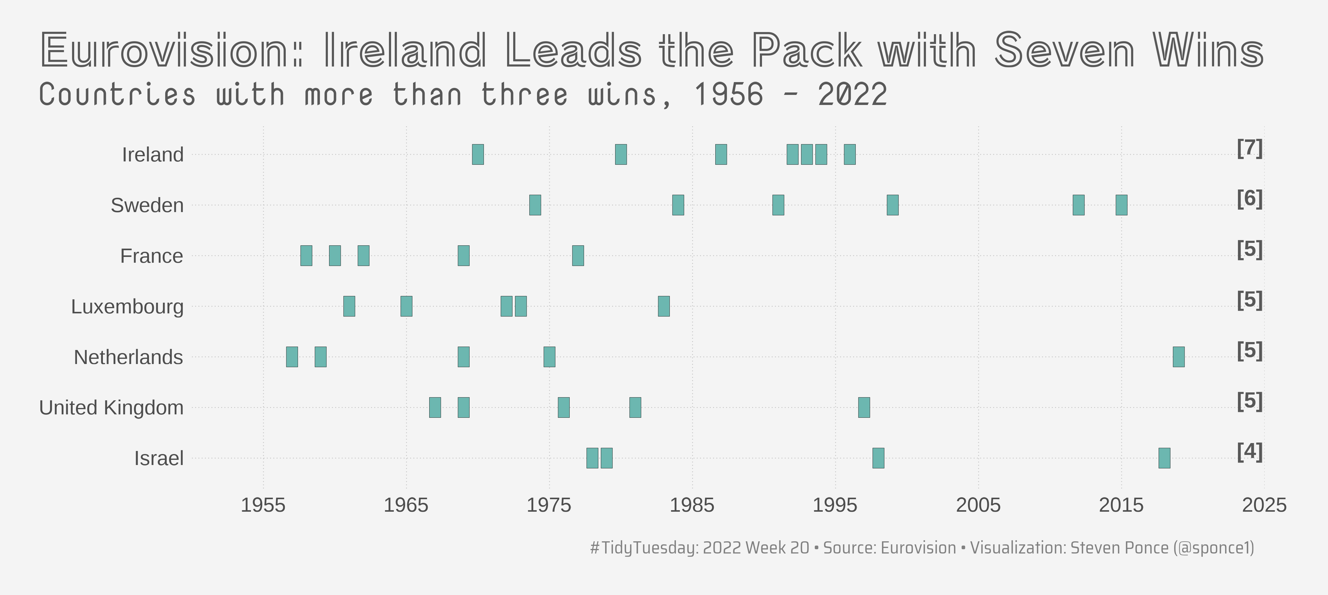{#fig-1}Additional information about this month's #SWDchallenge can be found [HERE](https://community.storytellingwithdata.com/challenges/nov-2024-make-a-good-graph)### Makeover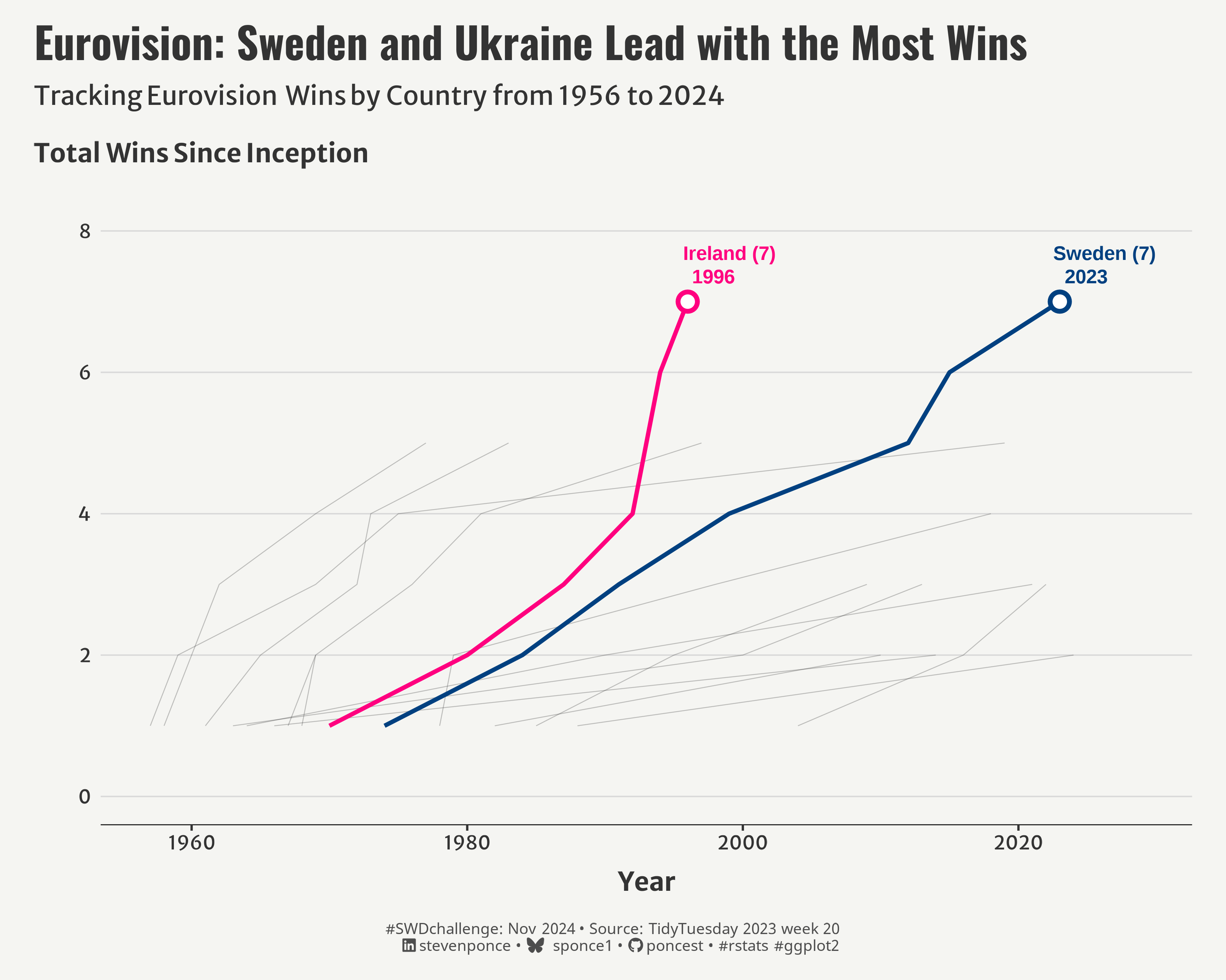{#fig-1}### <mark> __Steps to Create this Graphic__ </mark>#### 1. Load Packages & Setup ```{r}#| label: loadif (!require("pacman")) install.packages("pacman")pacman::p_load( tidyverse, # Easily Install and Load the 'Tidyverse' ggtext, # Improved Text Rendering Support for 'ggplot2' showtext, # Using Fonts More Easily in R Graphs janitor, # Simple Tools for Examining and Cleaning Dirty Data skimr, # Compact and Flexible Summaries of Data scales, # Scale Functions for Visualization glue, # Interpreted String Literals here, # A Simpler Way to Find Your Files tidytuesdayR, # Access the Weekly 'TidyTuesday' Project Dataset ggrepel # Automatically Position Non-Overlapping Text Labels with 'ggplot2') ### |- figure size ---- camcorder::gg_record( dir = here::here("temp_plots"), device ="png",width =10,height =8,units ="in",dpi =320)### |- resolution ---- showtext_opts(dpi =320, regular.wt =300, bold.wt =800)```#### 2. Read in the Data ```{r}#| label: readeurovision <- tidytuesdayR::tt_load(2022, week =20)$eurovision %>%clean_names() ```#### 3. Examine the Data```{r}#| label: examineglimpse(eurovision)skim(eurovision)colnames(eurovision)```#### 4. Tidy Data ```{r}#| label: tidy# Winners from 1956 to 2003winners_1956_2003_tbl <- eurovision |>filter(year <2004, section =='final', winner ==TRUE) |>select(year, host_city, artist_country, total_points, winner) |>arrange(desc(year)) |>drop_na()# Winners from 2004 to 2022winners_2004_2022_tbl <- eurovision |>filter(section =='grand-final', winner ==TRUE) |>select(year, host_city, artist_country, total_points, winner) |>arrange(desc(year)) |>drop_na()# Winners for 2023 and 2024winners_2023_2024_tbl <-tibble(year =c(2023, 2024),host_city =c("Liverpool", "Malmö"), artist_country =c("Sweden", "Switzerland"),total_points =c(583, 591), # Placeholder points, adjust based on real data if availablewinner =TRUE)# Combine all winnerswinners_combined_tbl <-bind_rows(winners_1956_2003_tbl, winners_2004_2022_tbl, winners_2023_2024_tbl) |>arrange(year) |>drop_na()# Calculate cumulative wins by yearcumulative_data <- winners_combined_tbl |>group_by(year, artist_country) |>summarise(total_points =sum(total_points), .groups ="drop") |>arrange(year) |>group_by(artist_country) |>mutate(cumulative_wins =row_number()) |>ungroup()# Define key countries to highlightkey_countries <-c("Sweden", "Ireland")# Get the most recent year for each key countrylatest_year_data <- cumulative_data |>filter(artist_country %in% key_countries) |>group_by(artist_country) |>filter(year ==max(year)) |>ungroup()```#### 5. Visualization Parameters ```{r}#| label: params### |- plot aesthetics ---- bkg_col <-"#f5f5f2"title_col <-"gray20"subtitle_col <-"gray20"caption_col <-"gray30"text_col <-"gray20"col_palette <-c("#FF007F", "#004080")### |- titles and caption ----# iconstt <-str_glue("#SWDchallenge: Nov 2024 • Source: TidyTuesday 2023 week 20<br>")li <-str_glue("<span style='font-family:fa6-brands'></span>")gh <-str_glue("<span style='font-family:fa6-brands'></span>")bs <-str_glue("<span style='font-family:fa6-brands'> </span>")title_text <-str_glue("Eurovision: Sweden and Ukraine Lead with the Most Wins")subtitle_text <-str_glue("Tracking Eurovision Wins by Country from 1956 to 2024<br><br> **Total Wins Since Inception**")caption_text <-str_glue("{tt} {li} stevenponce • {bs} sponce1 • {gh} poncest • #rstats #ggplot2")# |- fonts ----font_add('fa6-brands', here::here("fonts/6.6.0/Font Awesome 6 Brands-Regular-400.otf"))font_add_google("Oswald", regular.wt =400, family ="title") font_add_google("Merriweather Sans", regular.wt =400, family ="subtitle")font_add_google("Merriweather Sans", regular.wt =400, family ="text") font_add_google("Noto Sans", regular.wt =400,family ="caption")showtext_auto(enable =TRUE) ### |- plot theme ----theme_set(theme_minimal(base_size =14, base_family ="text")) theme_update(plot.title.position ="plot",plot.caption.position ="plot",legend.position ="plot",plot.background =element_rect(fill = bkg_col, color = bkg_col),panel.background =element_rect(fill = bkg_col, color = bkg_col),plot.margin =margin(t =10, r =20, b =10, l =20),axis.title.x =element_text(margin =margin(10, 0, 0, 0), size =rel(1.1), color = text_col, family ="text", face ="bold", hjust =0.5),axis.title.y =element_text(margin =margin(0, 10, 0, 0), size =rel(1.1), color = text_col, family ="text", face ="bold", hjust =0.5),axis.text =element_text(size =rel(0.8), color = text_col, family ="text"),axis.line.x =element_line(color ="#252525", linewidth = .3),axis.ticks.x =element_line(color = text_col), axis.title =element_text(face ="bold"),panel.grid.minor =element_blank(),panel.grid.major =element_blank(),panel.grid.major.y =element_line(color ="grey85", linewidth = .4),) ```#### 6. Plot```{r}#| label: plot# Line Chart cumulative_line_chart <-# Geomsggplot( cumulative_data,aes(x = year, y = cumulative_wins, group = artist_country, color = artist_country) ) +geom_line(data = cumulative_data |>filter(!artist_country %in% key_countries),linewidth =0.25, color ="gray20", alpha =0.3, linetype ="solid" ) +geom_line(data = cumulative_data |>filter(artist_country %in% key_countries),linewidth =1.2 ) +geom_point(data = latest_year_data,aes(color = artist_country), size =4, shape =21, fill ="white", stroke =2 ) +geom_text(data = latest_year_data,aes(label =str_glue("{artist_country} ({cumulative_wins})\n{year}")),vjust =-0.5,hjust =0.2, nudge_x =1, size =4, fontface ="bold", lineheight =1 ) +# Scalesscale_x_continuous(breaks =pretty_breaks(n =5),limits =c(min(cumulative_data$year), max(cumulative_data$year) +5) ) +scale_y_continuous(breaks =seq(0, 8, by =2),limits =c(0, 8) )+scale_color_manual(values = col_palette) +coord_cartesian(clip ="off") +# Labslabs(x ="Year",y ="",color ="Country",title = title_text,subtitle = subtitle_text,caption = caption_text ) +# Themetheme(plot.title =element_text(size =rel(1.8),family ="title",face ="bold",color = title_col,lineheight =1.1,margin =margin(t =5, b =5) ),plot.subtitle =element_markdown(size =rel(1.1),family ="subtitle",color = subtitle_col,lineheight =1.1,margin =margin(t =5, b =20) ),plot.caption =element_markdown(size =rel(0.65),family ="caption",color = caption_col,lineheight =1.1,hjust =0.5,halign =1,margin =margin(t =15, b =5) ) )# Show plotcumulative_line_chart```#### 7. Save```{r}#| label: save### |- plot image ---- # Save the plot againggsave(filename = here::here("data_visualizations/SWD Challenge/2024/swd_2024_11.png"),plot = cumulative_line_chart,width =10,height =8,units ="in",dpi =320)### |- plot thumbnail---- magick::image_read(here::here("data_visualizations/SWD Challenge/2024/swd_2024_11.png")) |> magick::image_resize(geometry ="400") |> magick::image_write(here::here("data_visualizations/SWD Challenge/2024/thumbnails/swd_2024_11.png"))```#### 8. Session Info::: {.callout-tip collapse="true"}##### Expand for Session Info```{r, echo = FALSE}#| eval: truesessionInfo()```:::#### 9. GitHub Repository::: {.callout-tip collapse="true"}##### Expand for GitHub Repo[Access the GitHub repository here](https://github.com/poncest/personal-website/):::

