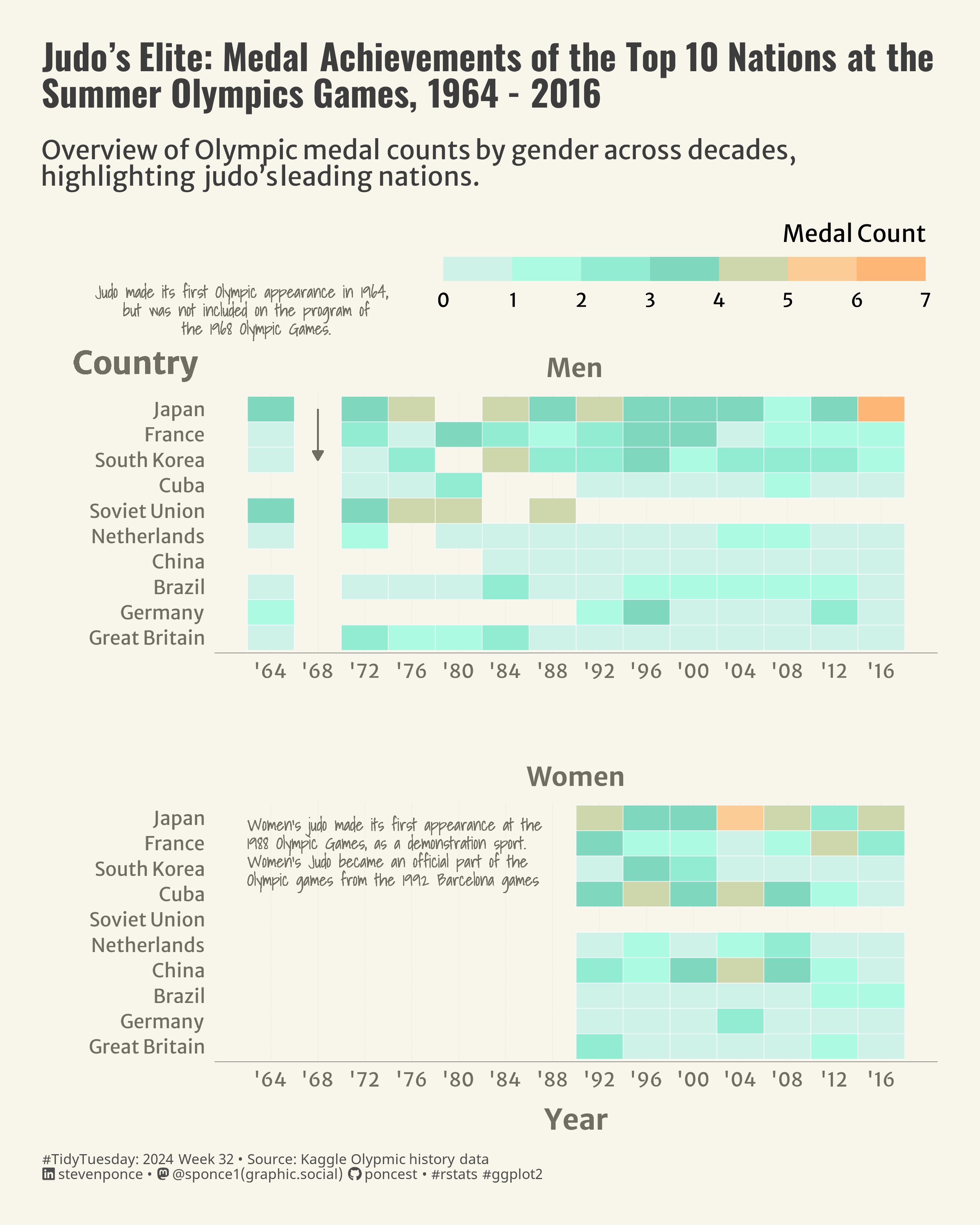
Judo’s Elite: Medal Achievements of the Top 10 Nations at the Summer Olympics Games, 1964 - 2016

Overview of Olympic medal counts by gender across decades, highlighting judo’s leading nations.

Figure 1: This heatmap illustrates the medal achievements of the top 10 nations in Olympic judo competitions from 1962 to 2016. The x-axis represents Olympic years, while the y-axis lists countries. The heatmap is divided into two sections: one for men and another for women. The colors on the heatmap range from light teal to dark orange, representing the number of medals won, from zero to seven, respectively.

Steps to Create this Graphic

1. Load Packages & Setup

```{r}
#| label: load

pacman::p_load(
  tidyverse,     # Easily Install and Load the 'Tidyverse'
  ggtext,        # Improved Text Rendering Support for 'ggplot2'
  showtext,      # Using Fonts More Easily in R Graphs
  janitor,       # Simple Tools for Examining and Cleaning Dirty Data
  skimr,         # Compact and Flexible Summaries of Data
  scales,        # Scale Functions for Visualization
  lubridate,     # Make Dealing with Dates a Little Easier
  MetBrewer      # Color Palettes Inspired by Works at the Metropolitan Museum of Art
 )  

### |- figure size ----
camcorder::gg_record(
  dir    = here::here("temp_plots"),
  device = "png",
  width  =  8,
  height =  10,
  units  = "in",
  dpi    = 320
)

### |- resolution ----
showtext_opts(dpi = 320, regular.wt = 300, bold.wt = 800)
```

2. Read in the Data

```{r}
#| label: read

tt <-tidytuesdayR::tt_load(2024, week = 32) 

olympics <- tt$olympics |> clean_names() |> glimpse()

tidytuesdayR::readme(tt)
rm(tt)
```

3. Examing the Data

```{r}
#| label: examine

glimpse(olympics)
skim(olympics)
```

4. Tidy Data

```{r}
#| label: tidy

# Judo df
judo <- olympics |> 
    filter(sport == "Judo") |> 
    mutate(
        gender = case_when(
            str_detect(event, "Men's")   ~ "Men",
            str_detect(event, "Women's") ~ "Women",
            TRUE ~ "Unspecified"  
        ),
        weight_class = str_replace_all(event, c("Men's " = "", "Women's " = "")),
        weight_class = str_replace_all(weight_class, c("Judo " = "")),
        weight_class = factor(weight_class, 
                              levels = c("Extra-Lightweight", "Half-Lightweight", "Lightweight", 
                                         "Half-Middleweight", "Middleweight" , "Half-Heavyweight", 
                                         "Heavyweight", "Open Class"))
        )  

# Judo medals
judo_medals <- judo |>
    filter(medal %in% c("Gold", "Silver", "Bronze")) |>
    count(country = team, year, gender, medal)

# Count medals for top countries
top_countries_medals <- judo_medals |>
    group_by(country) |>
    summarize(total_medals = sum(n)) |>
    slice_max(total_medals, n = 10) |>
    pull(country)

# Filter for the top 10 countries and calculate medals count
filtered_judo_medals <- judo |>
    filter(team %in% top_countries_medals) |>
    group_by(country = team, year, gender) |>
    summarise(
        medal_count = sum(medal %in% c("Gold", "Silver", "Bronze")), 
        .groups = "drop"
        ) |>
    arrange(country, year, gender)
```

5. Visualization Parameters

```{r}
#| label: params

### |- plot aesthetics ----
bkg_col      <- colorspace::lighten('#f7f5e9', 0.05)    
title_col    <- "#3d3d3d"           
subtitle_col <- "#3d3d3d"     
caption_col  <- "gray30"   
text_col     <- colorspace::darken("#8e8a7b" , 0.2)   

### |-  titles and caption ----
# icons
tt <- str_glue("#TidyTuesday: { 2024 } Week { 32 } &bull; Source: Kaggle Olypmic history data <br>")
li <- str_glue("<span style='font-family:fa6-brands'>&#xf08c;</span>")
gh <- str_glue("<span style='font-family:fa6-brands'>&#xf09b;</span>")
mn <- str_glue("<span style='font-family:fa6-brands'>&#xf4f6;</span>")

# text
title_text    <- str_glue("Judo’s Elite: Medal Achievements of the Top 10 Nations at the<br>
                          Summer Olympics Games, 1964 - 2016")
subtitle_text <- str_glue("Overview of Olympic medal counts by gender across decades,<br>
                          highlighting judo's leading nations.")
caption_text  <- str_glue("{tt} {li} stevenponce &bull; {mn} @sponce1(graphic.social) {gh} poncest &bull; #rstats #ggplot2")


### |-  fonts ----
font_add("fa6-brands", "fonts/6.4.2/Font Awesome 6 Brands-Regular-400.otf")
font_add_google("Oswald", regular.wt = 400, family = "title")
font_add_google("Merriweather Sans", regular.wt = 400, family = "subtitle")
font_add_google("Merriweather Sans", regular.wt = 400, family = "text")
font_add_google("Noto Sans", regular.wt = 400, family = "caption")
font_add_google("Shadows Into Light", regular.wt = 400, family = "anotation")
showtext_auto(enable = TRUE)


### |-  plot theme ----
theme_set(theme_minimal(base_size = 14, base_family = "text"))                

theme_update(
    plot.title.position   = "plot",
    plot.caption.position = "plot",
    legend.position       = 'top',
    legend.justification  = "right",
    legend.title.position = "top",
    legend.title.align    = 1,  
    legend.box.just       = "right",  
    
    plot.background       = element_rect(fill = bkg_col, color = bkg_col),
    panel.background      = element_rect(fill = bkg_col, color = bkg_col),
    plot.margin           = margin(t = 20, r = 25, b = 20, l = 25),
    axis.title.x          = element_text(margin = margin(10, 0, 0, 0), size = rel(1.2), 
                                         color = text_col, family = "text", face = "bold", hjust = 0.5),
    axis.title.y          = element_text(margin = margin(0, 10, 0, 0), size = rel(1.2), 
                                         color = text_col, family = "text", face = "bold", hjust = 0.5),
    axis.text             = element_text(size = rel(0.8), color = text_col, family = "text"),
    axis.line.x           = element_line(color = "gray40", linewidth = .15),
    panel.grid.minor.x    = element_blank(),
    panel.grid.major.x    = element_line(linetype = "dotted", linewidth = 0.1, color = 'gray'),
    panel.grid.minor.y    = element_blank(),
    panel.grid.major.y    = element_blank(),
    
    strip.text            = element_textbox(size     = rel(1.1),
                                            face     = 'bold',
                                            color    = text_col,
                                            hjust    = 0.5,
                                            halign   = 0.5,
                                            r        = unit(5, "pt"),
                                            width    = unit(5.5, "npc"),
                                            padding  = margin(3, 0, 3, 0),
                                            margin   = margin(3, 3, 3, 3),
                                            fill     = "transparent"),
    
    panel.spacing       = unit(3, 'lines'),
)  
```

6. Plot

```{r}
#| label: plot

### |-  initial plot ----  
p <- filtered_judo_medals |>
    ggplot(aes(x = year, y = fct_reorder(country, medal_count, .fun = sum), fill = medal_count)) +
    
  # Geoms
  geom_tile(color = "white", linewidth = 0.15) +
  geom_text(data = filtered_judo_medals |> filter(gender == "Men"),
            aes(label = "Country", x = 1962, y = "Japan"),
            size = 6.5, color = text_col, family = "text", fontface = "bold", 
            hjust = 1.4, vjust = -1.5) +

  # Scales
  scale_x_continuous(breaks = seq(
      min(filtered_judo_medals$year), 
      max(filtered_judo_medals$year), 
      by = 4), 
      labels = function(x) paste0("'", substr(x, 3, 4))) +
  scale_y_discrete() +
  coord_cartesian(clip = "off") +
  scale_fill_stepsn(
    colors = c('#DFEDEB', "#A1FCDF", "#7FD8BE", "#FCD29F", "#FCAB64"),
    limits = c(0, 7), 
    breaks = 0:7,
    labels = as.character(0:7),
    guide = guide_colorsteps(
        direction = "horizontal",
        barwidth = unit(10, "cm"),
        barheight = unit(0.5, "cm"),
        frame.colour = NA,
        title.position = "top",
        title.hjust = 1
        )
    ) +

  # Labs
  labs(
    title    = title_text,
    subtitle = subtitle_text,
    caption  = caption_text,
    x = "Year",
    y = "",
    fill = "Medal Count"
    ) +

  # Facet
  facet_wrap(vars(gender), nrow = 2, axes = "all") +

  # Theme
  theme(
      plot.title      = element_markdown(
          size        = rel(1.5),
          family      = "title",
          color       = title_col,
          face        = "bold",
          lineheight  = 0.85,
          margin      = margin(t = 5, b = 10)
      ),
      plot.subtitle   = element_markdown(
          size        = rel(1.1),
          family      = "subtitle",
          color       = title_col,
          lineheight  = 1,
          margin      = margin(t = 5, b = 10)
      ),
      plot.caption    = element_markdown(
          size        = rel(.6),
          family      = "caption",
          color       = caption_col,
          lineheight  = 0.6,
          hjust       = 0,
          halign      = 0,
          margin      = margin(t = 10, b = 5)
      ),
  )  
    
### |-  annotated plot ----  

men_text <- str_glue("Judo made its first Olympic appearance in 1964,\nbut was not included on the program of\nthe 1968 Olympic Games.")

women_text <- str_glue("Women's judo made its first appearance at the\n1988 Olympic Games, as a demonstration sport.\nWomen's Judo became an official part of the\nOlympic games from the 1992 Barcelona games")

### |-  final plot ----  
p <- p + 
    
    # Men's Judo History Note
    geom_text(data = filtered_judo_medals |> filter(gender == "Men"),
              aes(x = 1964, y = Inf, label = men_text),
              hjust = .6, vjust = -1.2, 
              size = 3.5, color = text_col,  family = "anotation", 
              lineheight = 0.9) +
    
    # Curved Arrow for Men's Note
    geom_curve(data = filtered_judo_medals |> filter(gender == "Men"),
               aes(x = 1968, y = "Japan", xend = 1968, yend = "South Korea"), 
               curvature = 0, arrow = arrow(type = "closed", length = unit(0.08, "inches")),
               linewidth = .5,  
               color = text_col, size = 0.7) +
    
    # Women's Judo History Note
    geom_text(data = filtered_judo_medals %>% filter(gender == "Women"),
              aes(label = women_text, x = 1962, y = "Japan"),
              hjust = 0, vjust = 1, size = 3.5, color = text_col, family = "anotation", 
              lineheight = 0.9) 
```

7. Save

```{r}
#| label: save

### |-  plot image ----  
ggsave(
  filename = here::here("data_visualizations/TidyTuesday/2024/tt_2024_32.png"),
  plot = p,
  width  =  8,
  height =  10,
  units  = "in",
  dpi    = 320
)

### |-  plot thumbnail----  
magick::image_read(here::here("data_visualizations/TidyTuesday/2024/tt_2024_32.png")) |> 
  magick::image_resize(geometry = "400") |> 
  magick::image_write(here::here("data_visualizations/TidyTuesday/2024/thumbnails/tt_2024_32.png"))
```

8. Session Info

```{r, eval=TRUE}
sessionInfo()
```

R version 4.4.1 (2024-06-14 ucrt)
Platform: x86_64-w64-mingw32/x64
Running under: Windows 11 x64 (build 22631)

Matrix products: default


locale:
[1] LC_COLLATE=English_United States.utf8 
[2] LC_CTYPE=English_United States.utf8   
[3] LC_MONETARY=English_United States.utf8
[4] LC_NUMERIC=C                          
[5] LC_TIME=English_United States.utf8    

time zone: America/New_York
tzcode source: internal

attached base packages:
[1] stats     graphics  grDevices datasets  utils     methods   base     

loaded via a namespace (and not attached):
 [1] htmlwidgets_1.6.4 compiler_4.4.0    fastmap_1.2.0     cli_3.6.4        
 [5] htmltools_0.5.8.1 tools_4.4.0       rstudioapi_0.17.1 yaml_2.3.10      
 [9] rmarkdown_2.29    knitr_1.49        jsonlite_1.8.9    xfun_0.49        
[13] digest_0.6.37     rlang_1.1.6       renv_1.0.3        evaluate_1.0.1