Character Interaction Networks in Shakespeare’s Plays

Visualizing character exchanges across different scenes and acts

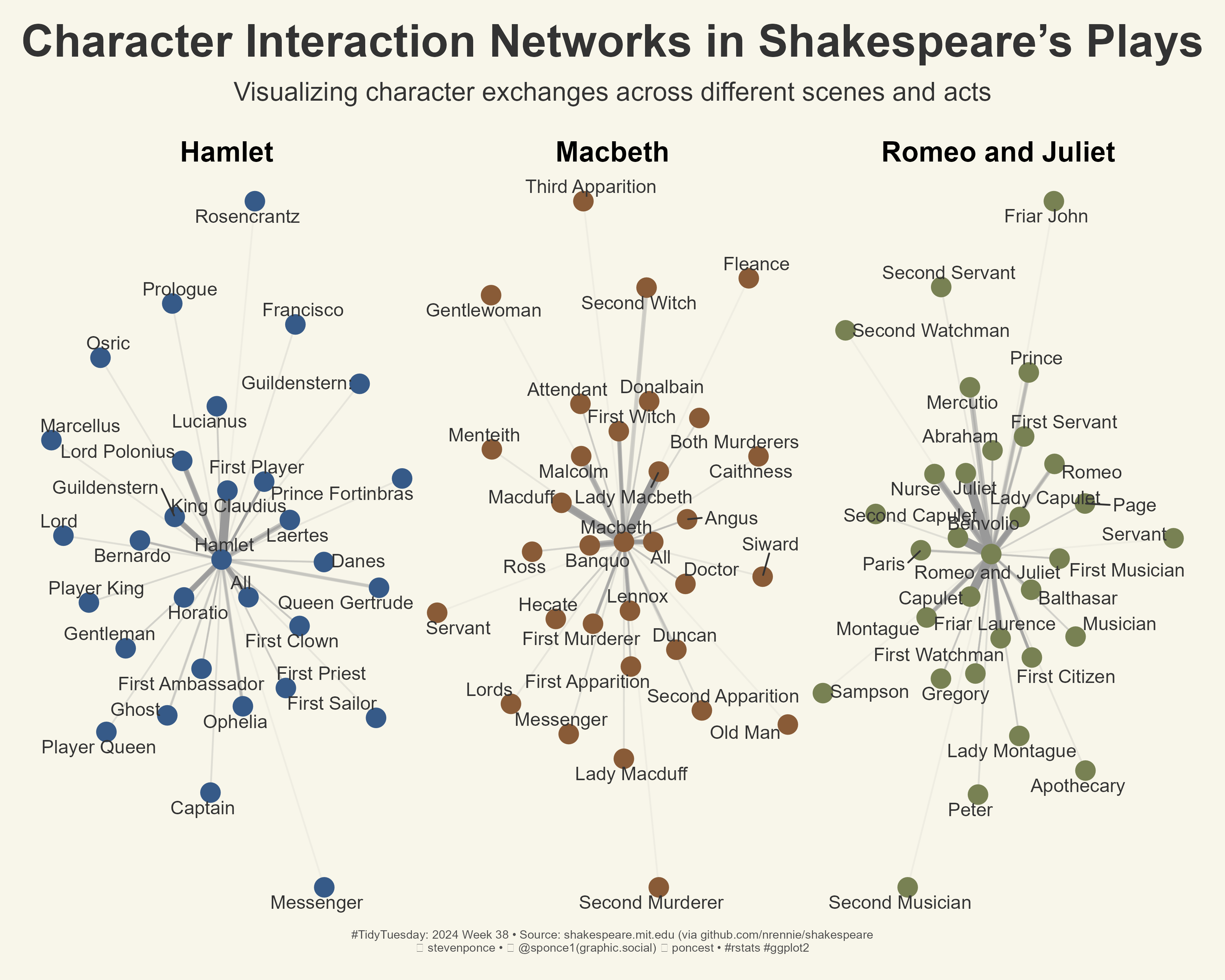
Figure 1: A visualization of character interaction networks in Shakespeare’s plays Hamlet, Macbeth, and Romeo and Juliet. The network plots display characters as nodes, with lines (edges) connecting characters who interact in the same scenes. Each plot has the title of the play centered above it. In Hamlet, nodes are blue; in Macbeth, they are brown; and in Romeo and Juliet, they are green.

Steps to Create this Graphic

1. Load Packages & Setup

```{r}
#| label: load

pacman::p_load(
  tidyverse,         # Easily Install and Load the 'Tidyverse'
  ggtext,            # Improved Text Rendering Support for 'ggplot2'
  showtext,          # Using Fonts More Easily in R Graphs
  janitor,           # Simple Tools for Examining and Cleaning Dirty Data
  skimr,             # Compact and Flexible Summaries of Data
  scales,            # Scale Functions for Visualization
  lubridate,         # Make Dealing with Dates a Little Easier
  MetBrewer,         # Color Palettes Inspired by Works at the Metropolitan Museum of Art
  MoMAColors,        # Color Palettes Inspired by Artwork at the Museum of Modern Art in New York City
  glue,              # Interpreted String Literals
  igraph,            # Network Analysis and Visualization # Network Analysis and Visualization # Network Analysis and Visualization # Network Analysis and Visualization
  ggraph,            # An Implementation of Grammar of Graphics for Graphs and Networks # An Implementation of Grammar of Graphics for Graphs and Networks # An Implementation of Grammar of Graphics for Graphs and Networks
  patchwork,         # The Composer of Plots
  NatParksPalettes   # Color Palettes Inspired by National Parks
 )  

# ### |- figure size ----
camcorder::gg_record(
  dir    = here::here("temp_plots"),
  device = "png",
  width  =  10,
  height =  8,
  units  = "in",
  dpi    = 320
)

### |- resolution ----
showtext_opts(dpi = 320, regular.wt = 300, bold.wt = 800)
```

2. Read in the Data

```{r}
#| label: read

tt <-tidytuesdayR::tt_load(2024, week = 38) 

hamlet <- tt$hamlet |> clean_names() |> glimpse()
macbeth <- tt$macbeth |> clean_names() |> glimpse()
romeo_juliet <- tt$romeo_juliet |> clean_names() |> glimpse()

tidytuesdayR::readme(tt)
rm(tt)
```

3. Examing the Data

```{r}
#| label: examine

glimpse(hamlet)
glimpse(macbeth)
glimpse(romeo_juliet)
```

4. Tidy Data

```{r}
#| label: tidy

# Preprocess data for character interactions
combined_plays <- bind_rows(
    hamlet |> mutate(play = "Hamlet"),
    macbeth |> mutate(play = "Macbeth"),
    romeo_juliet |> mutate(play = "Romeo and Juliet")
)

# Filter out stage directions
dialogue_data <- combined_plays |>
    filter(character != "[stage direction]") |>
    group_by(play, act, scene, character) |>
    summarize(dialogue = n(), .groups = 'drop')

# Filter out scenes with fewer than 2 characters
filtered_dialogue_data <- dialogue_data |>
    group_by(play, act, scene) |>
    filter(n() > 1) |> 
    ungroup()

# Create edges: character exchanges within the same scene
edges <- filtered_dialogue_data |>
    group_by(play, act, scene) |>
    summarise(pairs = list(combn(character, 2, simplify = FALSE)), .groups = 'drop') |>
    unnest(pairs) |>
    unnest_wider(pairs, names_sep = "_") |>
    rename(from = pairs_1, to = pairs_2) |>
    count(play, from, to) |> 
    rename(from_char = from, to_char = to)  # Rename columns to prevent conflicts

# Filter the data by each play and create separate graphs
hamlet_edges <- edges |> filter(play == "Hamlet")
macbeth_edges <- edges |> filter(play == "Macbeth")
romeo_juliet_edges <- edges |> filter(play == "Romeo and Juliet")

# Create separate igraph objects for each play
g_hamlet <- graph_from_data_frame(hamlet_edges, directed = FALSE)
g_macbeth <- graph_from_data_frame(macbeth_edges, directed = FALSE)
g_romeo_juliet <- graph_from_data_frame(romeo_juliet_edges, directed = FALSE)
```

5. Visualization Parameters

```{r}
#| label: params

### |- plot aesthetics ----
bkg_col      <- colorspace::lighten('#f7f5e9', 0.05)    
title_col    <- "gray20"           
subtitle_col <- "gray20"     
caption_col  <- "gray30"   
text_col     <- "gray20"    
col_palette  <- NatParksPalettes::natparks.pals(name = 'CraterLake', n = 3, type = "discrete")
col_palette  <- colorspace::lighten(col_palette, 0.1) 


### |-  titles and caption ----
# icons
tt <- str_glue("#TidyTuesday: { 2024 } Week { 38 } &bull; Source: shakespeare.mit.edu (via github.com/nrennie/shakespeare<br>")
li <- str_glue("<span style='font-family:fa6-brands'>&#xf08c;</span>")
gh <- str_glue("<span style='font-family:fa6-brands'>&#xf09b;</span>")
mn <- str_glue("<span style='font-family:fa6-brands'>&#xf4f6;</span>")

# text
title_text    <- str_glue("Character Interaction Networks in Shakespeare's Plays")
subtitle_text <- str_glue("Visualizing character exchanges across different scenes and acts")
caption_text  <- str_glue("{tt} {li} stevenponce &bull; {mn} @sponce1(graphic.social) {gh} poncest &bull; #rstats #ggplot2")

### |-  fonts ----
font_add("fa6-brands", "fonts/6.4.2/Font Awesome 6 Brands-Regular-400.otf")
font_add_google("Oswald", regular.wt = 400, family = "title")
font_add_google("Merriweather Sans", regular.wt = 400, family = "subtitle")
font_add_google("Merriweather Sans", regular.wt = 400, family = "text")
font_add_google("Noto Sans", regular.wt = 400, family = "caption")
showtext_auto(enable = TRUE)

### |-  plot theme ----
theme_set(theme_void(base_size = 14, base_family = "text"))                

theme_update(
    plot.title.position   = "plot",
    plot.caption.position = "plot",
    legend.position       = 'plot',
    plot.background       = element_rect(fill = bkg_col, color = bkg_col),
    panel.background      = element_rect(fill = bkg_col, color = bkg_col),
    plot.margin           = margin(t = 10, r = 20, b = 10, l = 20),
    strip.text            = element_textbox(size     = rel(1),
                                            face     = 'bold',
                                            color    = text_col,
                                            hjust    = 0.5,
                                            halign   = 0.5,
                                            r        = unit(3, "pt"),
                                            width    = unit(6, "npc"),
                                            padding  = margin(2, 0, 2, 0),
                                            margin   = margin(3, 3, 3, 3),
                                            fill     = "transparent"),
    panel.spacing         = unit(1, 'lines')
)  

### |-  plot function ----
plot_character_network <- function(play_name, edges_data, node_color, edge_color) {
    
    # Create igraph object for the play
    g_play <- graph_from_data_frame(edges_data, directed = FALSE)
    
    # Network plot
    plot <- ggraph(g_play, layout = 'fr') +
        geom_edge_link(aes(edge_alpha = n, edge_width = n), color = edge_color, show.legend = FALSE) +  # Set edge color with alpha and width
        geom_node_point(size = 5, color = node_color) +  # Set node color
        geom_node_text(aes(label = name), color = text_col, repel = TRUE, check_overlap = TRUE) +
        scale_edge_width(range = c(0.5, 2.5)) +
        theme_void() +
        ggtitle(play_name) +  # Add top-center title for the play
        theme(
            plot.title = element_text(size = rel(1.5), face = "bold", hjust = 0.5)  # Centered title with bold font
        )
    
    return(plot)
} 
```

6. Plot

```{r}
#| label: plot

### |-  individual plots ----
hamlet_plot       <- plot_character_network("Hamlet", hamlet_edges, node_color = col_palette[1], edge_color = "gray60")
macbeth_plot      <- plot_character_network("Macbeth", macbeth_edges, node_color = col_palette[2], edge_color = "gray60")
romeo_juliet_plot <- plot_character_network("Romeo and Juliet", romeo_juliet_edges, col_palette[3], edge_color = "gray60")

### |-  Combine plots using patchwork ----
combined_plot <- hamlet_plot + macbeth_plot + romeo_juliet_plot + 
    patchwork::plot_layout(ncol = 3)

### |-  final plot ----  
final_plot <- combined_plot + 
    plot_annotation(
        title = title_text,
        subtitle = subtitle_text,
        caption = caption_text,
        
        # Theme
        theme = theme(
            plot.title        = element_markdown(
                size          = rel(1.9),   
                hjust         = 0.5,
                family        = "title",
                face          = "bold",
                color         = title_col,
                lineheight    = 1.1,
                margin        = margin(t = 5, b = 5)
            ),
            plot.subtitle     = element_markdown(
                size          = rel(1.1), 
                hjust         = 0.5,
                family        = 'subtitle',
                color         = subtitle_col,
                lineheight    = 1.1, 
                margin        = margin(t = 5, b = 15)
            ),
            plot.caption      = element_markdown(
                size          = rel(.50),
                family        = "caption",
                color         = caption_col,
                lineheight    = 1.1,
                hjust         = 0.5,
                halign        = 0.5,
                margin        = margin(t = 5, b = 5)
            ),
        )
    )
```

7. Save

```{r}
#| label: save

### |-  plot image ----  

library(ggplotify)
# Convert patchwork plot to grob 
# There was some issues between patchwork and ggsave
plot_grob <- as.grob(final_plot)

# Save the plot again
ggsave(
    filename = here::here("data_visualizations/TidyTuesday/2024/tt_2024_38.png"),
    plot = plot_grob,
    width  = 10,
    height = 8,
    units  = "in",
    dpi    = 320
)

### |-  plot thumbnail----  
magick::image_read(here::here("data_visualizations/TidyTuesday/2024/tt_2024_38.png")) |> 
  magick::image_resize(geometry = "400") |> 
  magick::image_write(here::here("data_visualizations/TidyTuesday/2024/thumbnails/tt_2024_38.png"))
```

8. Session Info

```{r, eval=TRUE}
sessionInfo()
```

R version 4.4.1 (2024-06-14 ucrt)
Platform: x86_64-w64-mingw32/x64
Running under: Windows 11 x64 (build 22631)

Matrix products: default


locale:
[1] LC_COLLATE=English_United States.utf8 
[2] LC_CTYPE=English_United States.utf8   
[3] LC_MONETARY=English_United States.utf8
[4] LC_NUMERIC=C                          
[5] LC_TIME=English_United States.utf8    

time zone: America/New_York
tzcode source: internal

attached base packages:
[1] stats     graphics  grDevices datasets  utils     methods   base     

loaded via a namespace (and not attached):
 [1] htmlwidgets_1.6.4 compiler_4.4.0    fastmap_1.2.0     cli_3.6.4        
 [5] htmltools_0.5.8.1 tools_4.4.0       rstudioapi_0.17.1 yaml_2.3.10      
 [9] rmarkdown_2.29    knitr_1.49        jsonlite_1.8.9    xfun_0.49        
[13] digest_0.6.37     rlang_1.1.6       renv_1.0.3        evaluate_1.0.1