Qatar Cars: A Modern, Global Dataset Reveals Four Market Segments

Price-power positioning from 105 vehicles shows distinct clustering from
budget ($12k-25k) through mid-range ($25k-75k) and premium ($75k-250k) to ultra-luxury ($250k+)

Exploring the Qatar Cars dataset—a modern, internationally-focused alternative to mtcars—through price-power positioning analysis. This scatter plot visualization reveals four distinct market segments and demonstrates how the dataset captures the full automotive spectrum from budget vehicles to multi-million dollar hypercars.

Figure 1: A scatter plot of 105 vehicles, plotted by price (USD, log-scale x-axis) versus horsepower (y-axis). Density contours reveal four distinct market segments divided by vertical lines: Budget ($12k-25k), Mid-Range ($25k-75k), Premium ($75k-250k), and Ultra-Luxury ($250k+). Points are colored by engine type (teal for electric, orange for hybrid, dark gray for petrol). The majority of vehicles cluster in the budget and mid-range segments below 500 horsepower. Four ultra-luxury outliers are labeled in the upper right: Lotus Evija ($2.2M), Bugatti Centodieci ($9.1M), Bugatti Chiron ($3.6M), and McLaren Senna ($1.4M).

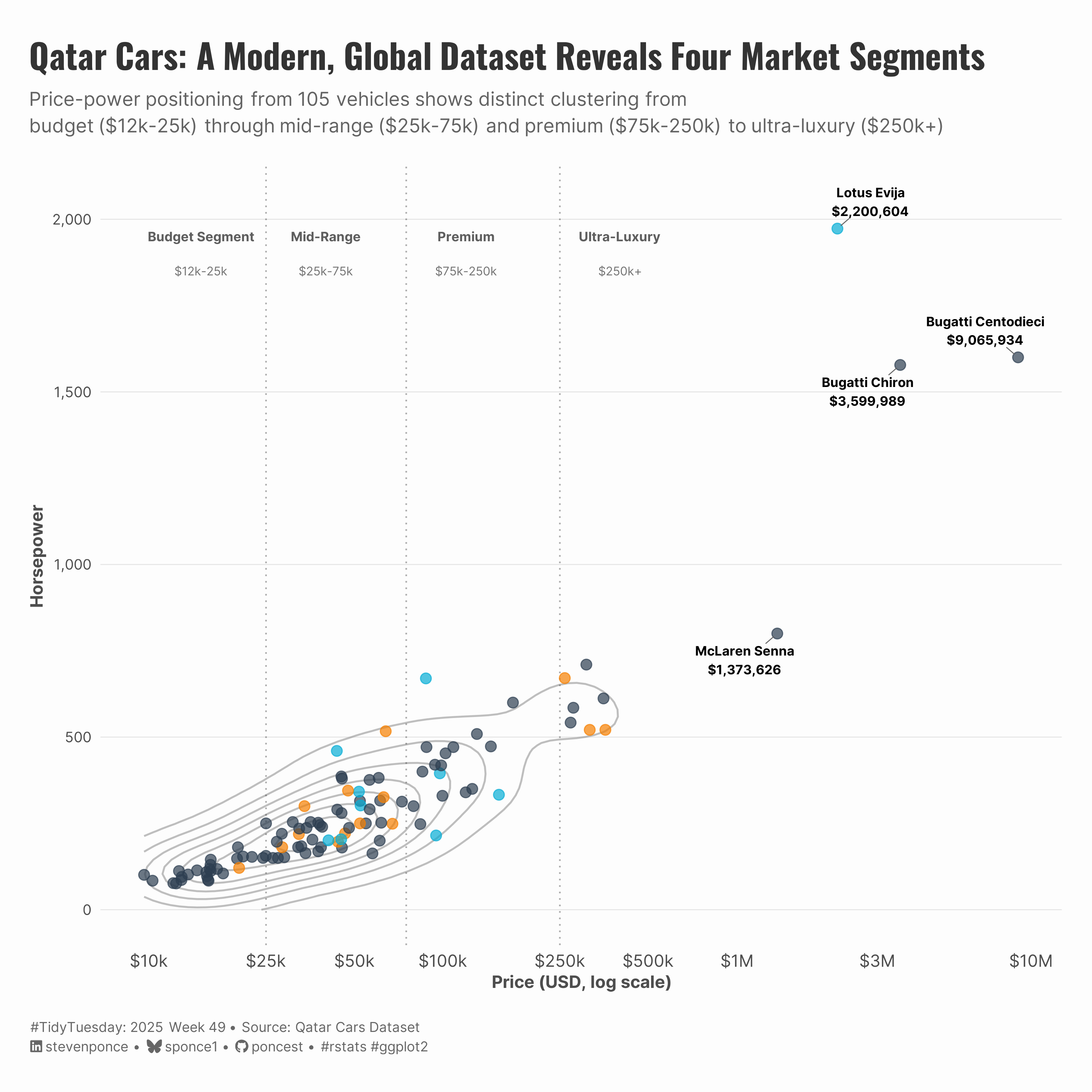Steps to Create this Graphic

1. Load Packages & Setup

```{r}
#| label: load
#| warning: false
#| message: false
#| results: "hide"

## 1. LOAD PACKAGES & SETUP ----
suppressPackageStartupMessages({
if (!require("pacman")) install.packages("pacman")
pacman::p_load(
    tidyverse,     # Easily Install and Load the 'Tidyverse'
    ggtext,        # Improved Text Rendering Support for 'ggplot2'
    showtext,      # Using Fonts More Easily in R Graphs
    janitor,       # Simple Tools for Examining and Cleaning Dirty Data
    scales,        # Scale Functions for Visualization
    glue,          # Interpreted String Literals
    ggrepel        # Automatically Position Non-Overlapping Text Labels
)
})

### |- figure size ----
camcorder::gg_record(
  dir    = here::here("temp_plots"),
  device = "png",
  width  = 10,
  height = 10,
  units  = "in",
  dpi    = 320
)

# Source utility functions
suppressMessages(source(here::here("R/utils/fonts.R")))
source(here::here("R/utils/social_icons.R"))
source(here::here("R/utils/image_utils.R"))
source(here::here("R/themes/base_theme.R"))
```

2. Read in the Data

```{r}
#| label: read
#| include: true
#| eval: true
#| warning: false

tt <- tidytuesdayR::tt_load(2025, week = 49)

qatarcars <- tt$qatarcars |> clean_names()

tidytuesdayR::readme(tt)
rm(tt)
```

3. Examine the Data

```{r}
#| label: examine
#| include: true
#| eval: true
#| results: 'hide'
#| warning: false

glimpse(qatarcars)
skimr::skim(qatarcars) |> summary()
```

4. Tidy Data

```{r}
#| label: tidy-fixed
#| warning: false

qatarcars_tidy <- qatarcars |>
  mutate(
    price_usd = price / 3.64,
    price_eur = price / 4.15
  )

# Identify top 4 most expensive cars
top4_cars <- qatarcars_tidy |>
  arrange(desc(price_usd)) |>
  head(4) |>
  mutate(
    label = paste0(make, " ", model, "\n$", label_comma(accuracy = 1)(price_usd))
  )

# Define market segments
segment_labels <- tibble(
  segment = c("Budget Segment", "Mid-Range", "Premium", "Ultra-Luxury"),
  price_usd = c(15000, 40000, 120000, 400000),
  horsepower = c(1950, 1950, 1950, 1950),
  price_range = c("$12k-25k", "$25k-75k", "$75k-250k", "$250k+")
)
```

5. Visualization Parameters

```{r}
#| label: params
#| include: true
#| warning: false

### |- plot aesthetics ----
colors <- get_theme_colors(
    palette = list(
        "Electric" = "#06AED5",
        "Hybrid" = "#F77F00", 
        "Petrol" = "#2C3E50",
        col_gray = "gray70"
    )
)

### |- titles and caption ----
title_text <- str_glue("Qatar Cars: A Modern, Global Dataset Reveals Four Market Segments")
subtitle_text <- str_glue(
    "Price-power positioning from 105 vehicles shows distinct clustering from<br>",
    "**budget** ($12k-25k) through **mid-range** ($25k-75k) and **premium** ($75k-250k) to **ultra-luxury** ($250k+)"
)

caption_text <- create_social_caption(
    tt_year  = 2025,
    tt_week  = 49,  
    source_text = str_glue(
        "Qatar Cars Dataset",
    )
)

### |-  fonts ----
setup_fonts()
fonts <- get_font_families()

### |-  plot theme ----
# Start with base theme
base_theme <- create_base_theme(colors)

# Add weekly-specific theme elements
weekly_theme <- extend_weekly_theme(
  base_theme,
  theme(
    # Text styling
    plot.title = element_markdown(
      face = "bold", family = fonts$title, size = rel(1.4),
      color = colors$title, margin = margin(b = 10), hjust = 0
    ),
    plot.subtitle = element_markdown(
      face = "italic", family = fonts$subtitle, lineheight = 1.2,
      color = colors$subtitle, size = rel(0.9), margin = margin(b = 20), hjust = 0
    ),

    # Grid
    panel.grid.minor = element_blank(),
    # panel.grid.major.x = element_blank(),
    panel.grid.major = element_line(color = "gray90", linewidth = 0.3),

    # Axes
    axis.title = element_text(size = rel(0.8), color = "gray30"),
    axis.text = element_text(color = "gray30"),
    axis.text.y = element_text(size = rel(0.85)),
    axis.ticks = element_blank(),

    # Facets
    strip.background = element_rect(fill = "gray95", color = NA),
    strip.text = element_text(
      face = "bold",
      color = "gray20",
      size = rel(0.9),
      margin = margin(t = 6, b = 4)
    ),
    panel.spacing = unit(1.5, "lines"),

    # Legend elements
    legend.position = "plot",
    legend.title = element_text(
      family = fonts$subtitle,
      color = colors$text, size = rel(0.8), face = "bold"
    ),
    legend.text = element_text(
      family = fonts$tsubtitle,
      color = colors$text, size = rel(0.7)
    ),
    legend.margin = margin(t = 15),

    # Plot margin
    plot.margin = margin(20, 20, 20, 20)
  )
)

# Set theme
theme_set(weekly_theme)
```

6. Plot

```{r}
#| label: plot
#| warning: false

# labeling function for x-axis (k for thousands, M for millions)
custom_dollar_labels <- function(x) {
    case_when(
        x >= 1e6 ~ paste0("$", x / 1e6, "M"),
        x >= 1e3 ~ paste0("$", x / 1e3, "k"),
        TRUE ~ paste0("$", x)
    )
}

### |-  main plot ----
p <- qatarcars_tidy |>
  ggplot(aes(x = price_usd, y = horsepower)) +
  # Geoms
  geom_density2d(color = "gray50", alpha = 0.5, linewidth = 0.6) +
  geom_vline(xintercept = 25000, linetype = "dotted", color = "gray20", alpha = 0.4) +
  geom_vline(xintercept = 75000, linetype = "dotted", color = "gray20", alpha = 0.4) +
  geom_vline(xintercept = 250000, linetype = "dotted", color = "gray20", alpha = 0.4) +
  geom_text(
    data = segment_labels,
    aes(x = price_usd, y = horsepower, label = segment),
    size = 3,
    fontface = "bold",
    color = "gray30",
    alpha = 0.9,
    family = fonts$text
  ) +
  geom_text(
    data = segment_labels,
    aes(x = price_usd, y = 1850, label = price_range),
    size = 2.8,
    color = "gray40",
    alpha = 0.9,
    family = fonts$text
  ) +
  geom_point(aes(color = enginetype), alpha = 0.7, size = 3) +
  geom_text_repel(
    data = top4_cars,
    aes(label = label),
    size = 3,
    fontface = "bold",
    box.padding = 0.5,
    point.padding = 0.3,
    segment.color = "gray40",
    segment.size = 0.3,
    min.segment.length = 0,
    family = fonts$text,
    seed = 1234
  ) +
  # Scales
  scale_x_log10(
    labels = custom_dollar_labels,
    breaks = c(10000, 25000, 50000, 100000, 250000, 500000, 1e6, 3e6, 10e6)
  ) +
  scale_y_continuous(labels = label_comma(), limits = c(0, 2050)) +
  scale_color_manual(
    values = colors$palette,
    name = "Engine Type"
  ) +
  # Labs
  labs(
    title = title_text,
    subtitle = subtitle_text,
    x = "Price (USD, log scale)",
    y = "Horsepower",
    caption = caption_text
  ) +
  # Theme
  theme(
    plot.title = element_markdown(
      size = rel(1.6),
      family = fonts$title,
      face = "bold",
      color = colors$title,
      lineheight = 1.15,
      margin = margin(t = 8, b = 5)
    ),
    plot.subtitle = element_markdown(
      size = rel(0.9),
      family = fonts$subtitle,
      color = alpha(colors$subtitle, 0.88),
      lineheight = 1.4,
      margin = margin(t = 5, b = 20)
    ),
    plot.caption = element_markdown(
      size = rel(0.65),
      family = fonts$subtitle,
      color = colors$caption,
      hjust = 0,
      lineheight = 1.4,
      margin = margin(t = 20, b = 5)
    ),
    panel.grid.minor.x = element_blank(),
    panel.grid.major.x = element_blank(),
  )
```

7. Save

```{r}
#| label: save
#| warning: false

### |-  plot image ----  
save_plot(
  plot = p, 
  type = "tidytuesday", 
  year = 2025, 
  week = 49, 
  width  = 10,
  height = 10,
  )
```

8. Session Info

Expand for Session Info

R version 4.4.1 (2024-06-14 ucrt)
Platform: x86_64-w64-mingw32/x64
Running under: Windows 11 x64 (build 26100)

Matrix products: default


locale:
[1] LC_COLLATE=English_United States.utf8 
[2] LC_CTYPE=English_United States.utf8   
[3] LC_MONETARY=English_United States.utf8
[4] LC_NUMERIC=C                          
[5] LC_TIME=English_United States.utf8    

time zone: America/New_York
tzcode source: internal

attached base packages:
[1] stats     graphics  grDevices datasets  utils     methods   base     

other attached packages:
 [1] here_1.0.1      ggrepel_0.9.6   glue_1.8.0      scales_1.3.0   
 [5] janitor_2.2.0   showtext_0.9-7  showtextdb_3.0  sysfonts_0.8.9 
 [9] ggtext_0.1.2    lubridate_1.9.3 forcats_1.0.0   stringr_1.5.1  
[13] dplyr_1.1.4     purrr_1.0.2     readr_2.1.5     tidyr_1.3.1    
[17] tibble_3.2.1    ggplot2_3.5.1   tidyverse_2.0.0 pacman_0.5.1   

loaded via a namespace (and not attached):
 [1] tidyselect_1.2.1   farver_2.1.2       fastmap_1.2.0      gh_1.4.1          
 [5] digest_0.6.37      timechange_0.3.0   lifecycle_1.0.4    rsvg_2.6.1        
 [9] magrittr_2.0.3     compiler_4.4.0     rlang_1.1.6        tools_4.4.0       
[13] utf8_1.2.4         yaml_2.3.10        knitr_1.49         skimr_2.1.5       
[17] labeling_0.4.3     htmlwidgets_1.6.4  bit_4.5.0          curl_6.0.0        
[21] xml2_1.3.6         camcorder_0.1.0    repr_1.1.7         tidytuesdayR_1.1.2
[25] withr_3.0.2        grid_4.4.0         fansi_1.0.6        colorspace_2.1-1  
[29] gitcreds_0.1.2     MASS_7.3-60.2      isoband_0.2.7      cli_3.6.4         
[33] rmarkdown_2.29     crayon_1.5.3       ragg_1.3.3         generics_0.1.3    
[37] rstudioapi_0.17.1  tzdb_0.5.0         commonmark_1.9.2   parallel_4.4.0    
[41] base64enc_0.1-3    vctrs_0.6.5        jsonlite_1.8.9     hms_1.1.3         
[45] bit64_4.5.2        systemfonts_1.1.0  magick_2.8.5       gifski_1.32.0-1   
[49] codetools_0.2-20   stringi_1.8.4      gtable_0.3.6       munsell_0.5.1     
[53] pillar_1.9.0       rappdirs_0.3.3     htmltools_0.5.8.1  R6_2.5.1          
[57] httr2_1.0.6        textshaping_0.4.0  rprojroot_2.0.4    vroom_1.6.5       
[61] evaluate_1.0.1     markdown_1.13      gridtext_0.1.5     snakecase_0.11.1  
[65] renv_1.0.3         Rcpp_1.0.13-1      svglite_2.1.3      xfun_0.49         
[69] pkgconfig_2.0.3   

9. GitHub Repository

Expand for GitHub Repo

The complete code for this analysis is available in tt_2025_49.qmd.

For the full repository, click here.

10. References

Expand for References

1. Data Source:
   • TidyTuesday 2025 Week 49: CCars in Qatar

11. Custom Functions Documentation

📦 Custom Helper Functions

This analysis uses custom functions from my personal module library for efficiency and consistency across projects.

Functions Used:

• fonts.R: setup_fonts(), get_font_families() - Font management with showtext
• social_icons.R: create_social_caption() - Generates formatted social media captions
• image_utils.R: save_plot() - Consistent plot saving with naming conventions
• base_theme.R: create_base_theme(), extend_weekly_theme(), get_theme_colors() - Custom ggplot2 themes

Why custom functions?
These utilities standardize theming, fonts, and output across all my data visualizations. The core analysis (data tidying and visualization logic) uses only standard tidyverse packages.

Source Code:
View all custom functions → GitHub: R/utils