IELTS Averages Barely Moved. Reading and Listening Scores Didn’t.

Change in mean IELTS band score by component, 2022-23 to 2024-25 cohorts.

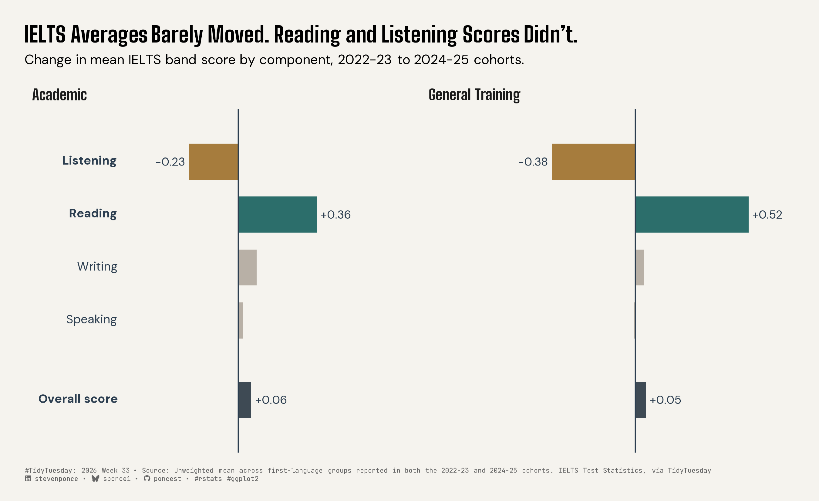
Change in mean IELTS band score between the 2022-23 and 2024-25 test-taker cohorts reveals that stable overall scores concealed a sharp divergence: Reading rose while Listening fell, in both Academic and General Training formats. The analysis is restricted to first-language groups reported in both cohorts, using an unweighted mean of per-language deltas. Built in R with ggplot2, ggtext, and ggview.

Figure 1: Two-panel diverging bar chart titled “IELTS Averages Barely Moved. Reading and Listening Scores Didn’t,” showing change in mean IELTS band score by component between the 2022-23 and 2024-25 cohorts, split by Academic and General Training exam formats. In both formats, Reading scores rose (Academic +0.36, General Training +0.52) while Listening scores fell (Academic -0.23, General Training -0.38), a mirrored pattern across both panels. Writing and Speaking barely changed in either format. Despite these offsetting shifts, the Overall score barely moved (Academic +0.06, General Training +0.05), as shown in the separate bar below the four skill components. Bars are colored by role: teal for Reading, ochre for Listening, warm gray for Writing and Speaking, and dark slate for the Overall aggregate. Source: IELTS Test Statistics, via TidyTuesday.

Steps to Create this Graphic

1. Load Packages & Setup

```{r}
#| label: load
#| warning: false
#| message: false      
#| results: "hide"     

## 1. LOAD PACKAGES & SETUP ----
suppressPackageStartupMessages({
if (!require("pacman")) install.packages("pacman")
pacman::p_load(
    tidyverse, ggtext, showtext, janitor, ggrepel,      
    scales, glue, skimr, ggview
    )
})

# Source utility functions
suppressMessages(source(here::here("R/utils/fonts.R")))
source(here::here("R/utils/social_icons.R"))
source(here::here("R/utils/image_utils.R"))
source(here::here("R/themes/base_theme.R"))
```

2. Read in the Data

```{r}
#| label: read
#| include: true
#| eval: true
#| warning: false

## 2. READ IN THE DATA ----
tt <- tidytuesdayR::tt_load(2026, week = 33)
perf_lang <- tt$performance_by_first_language
# demo_by_first_language <- tt$demo_by_first_language
# demo_by_nationality <- tt$demo_by_nationality
# demo_by_reasons <- tt$demo_by_reasons
# performance_by_nationality <- tt$performance_by_nationality
rm(tt)
```

3. Examine the Data

```{r}
#| label: examine
#| include: true
#| eval: true
#| results: 'hide'
#| warning: false

## 3. EXAMINING THE DATA ----
glimpse(perf_lang)
skim_without_charts(perf_lang)
distinct(perf_lang, year)
distinct(perf_lang, part)
```

4. Tidy Data

```{r}
#| label: tidy
#| warning: false

### |- harmonize cross-cohort spelling/label drift ----
language_harmonize <- c(
  "Gujurati"   = "Gujarati",
  "Ibo/lgbo"   = "Ibo/Igbo",
  "Singhalese" = "Sinhalese"
)

perf_lang_clean <- perf_lang |>
  mutate(language = recode(language, !!!language_harmonize))

### |- restrict to languages present in BOTH comparison cohorts ----
## robustness check already run in Phase 0.
languages_both_cohorts <- perf_lang_clean |>
  filter(year %in% c("2022-2023", "2024-2025")) |>
  distinct(type, language, year) |>
  count(type, language) |>
  filter(n == 2) |>
  distinct(type, language)

matched_scores <- perf_lang_clean |>
  filter(year %in% c("2022-2023", "2024-2025")) |>
  mutate(part = str_to_title(part)) |>
  semi_join(languages_both_cohorts, by = c("type", "language"))

### |- aggregate spine: mean of per-language deltas, matched languages only ----
per_language_delta <- matched_scores |>
  pivot_wider(
    id_cols = c(type, language, part),
    names_from = year, values_from = score
  ) |>
  mutate(delta = `2024-2025` - `2022-2023`)

### |- y_pos ----
component_positions <- tibble::tibble(
  part  = c("Overall", "Speaking", "Writing", "Reading", "Listening"),
  label = c("Overall score", "Speaking", "Writing", "Reading", "Listening"),
  y_pos = c(1, 2.5, 3.5, 4.5, 5.5)
)

## Row labels
label_data <- component_positions |>
  mutate(
    label = if_else(
      part %in% c("Overall", "Reading", "Listening"),
      str_glue("**{label}**"),
      label
    ),
    type_label = "Academic"
  )

delta_data <- per_language_delta |>
  summarise(delta = mean(delta, na.rm = TRUE), .by = c(type, part)) |>
  mutate(
    role = case_when(
      part == "Reading" ~ "reading",
      part == "Listening" ~ "listening",
      part == "Overall" ~ "overall",
      TRUE ~ "context"
    ),
    type_label = if_else(
      type == "General_Training", "General Training", "Academic"
    ),
    label_this = part %in% c("Reading", "Listening", "Overall")
  ) |>
  left_join(component_positions, by = "part") |>
  arrange(type, y_pos)
```

5. Visualization Parameters

```{r}
#| label: params
#| include: true
#| warning: false

### |-  plot aesthetics ----
colors <- get_theme_colors(
  palette = list(
    reading   = "#2C6E6B",
    listening = "#A67C3D",
    context   = "#B8B0A6",
    overall   = "#3E4A54"
  )
)

### |- titles and caption ----
title_text <- str_glue("IELTS Averages Barely Moved. Reading and Listening Scores Didn't.")

subtitle_text <- str_glue("Change in mean IELTS band score by component, 2022-23 to 2024-25 cohorts.")

caption_text <- create_social_caption(
  tt_year = 2026,
  tt_week = 33,
  source_text = str_glue(
    "Unweighted mean across first-language groups reported in both the ",
    "2022-23 and 2024-25 cohorts. IELTS Test Statistics, via TidyTuesday"
  )
)

### |-  fonts ----
setup_fonts()
fonts <- get_font_families()

### |-  plot theme ----
base_theme <- create_base_theme(colors)

weekly_theme <- extend_weekly_theme(
  base_theme,
  theme(
    plot.title = element_textbox_simple(
      face = "bold", family = fonts$title_1,
      size = 16, lineheight = 1.2,
      margin = margin(b = 6)
    ),
    plot.subtitle = element_textbox_simple(
      family = fonts$subtitle, size = 10,
      lineheight = 1.3,
      margin = margin(b = 10)
    ),
    plot.caption = element_textbox_simple(
      family = fonts$caption, size = 5,
      color = "gray40", lineheight = 1.3,
      margin = margin(t = 12)
    ),
    plot.margin = margin(t = 20, r = 20, b = 15, l = 20),
    strip.text = element_text(
      face = "bold", family = fonts$title_1, size = 11, hjust = 0
    ),
    panel.grid = element_blank(),
    axis.ticks = element_blank(),
    axis.text.y = element_blank(),
    axis.text.x = element_blank(),
    axis.title = element_blank(),
    legend.position = "none",
    panel.spacing.x = unit(1.4, "lines")
  )
)

theme_set(weekly_theme)
```

6. Plot

```{r}
#| label: plot
#| warning: false
### |-  plot ----
p <- delta_data |>
  ggplot(aes(x = delta, y = y_pos, fill = role)) +
  geom_col(width = 0.68, orientation = "y", na.rm = TRUE) +
  geom_vline(xintercept = 0, color = "#2C3E50", linewidth = 0.4) +
  geom_richtext(
    data = label_data,
    aes(x = -0.55, y = y_pos, label = label),
    inherit.aes = FALSE,
    hjust = 1, size = 3.2, color = "#2C3E50",
    family = fonts$subtitle,
    fill = NA, label.color = NA,
    label.padding = unit(0, "pt")
  ) +
  geom_text(
    data = filter(delta_data, label_this),
    aes(
      label = label_number(style_positive = "plus", accuracy = 0.01)(delta),
      hjust = if_else(delta >= 0, -0.15, 1.15)
    ),
    size = 3, family = fonts$subtitle, color = "#2C3E50"
  ) +
  facet_wrap(~type_label, nrow = 1) +
  coord_cartesian(clip = "off") +
  scale_x_continuous(limits = c(-0.9, 0.65)) +
  scale_y_continuous(breaks = NULL, limits = c(0.3, 6.2)) +
  scale_fill_manual(
    values = c(
      reading   = "#2C6E6B",
      listening = "#A67C3D",
      context   = "#B8B0A6",
      overall   = "#3E4A54"
    ),
    na.value = NA
  ) +
  labs(
    title = title_text,
    subtitle = subtitle_text,
    caption = caption_text,
    x = NULL, y = NULL
  )
```

7. Save

```{r}
#| label: save
#| warning: false

### |- save ----
main_path  <- here::here("data_visualizations", "TidyTuesday", "2026", "tt_2026_33.png")
thumb_path <- here::here("data_visualizations", "TidyTuesday", "2026", "thumbnails", "tt_2026_33.png")

# Full-size version, for the QMD figure
save_ggplot(
  plot = p,
  file = main_path,
  width = 9,
  height = 5.5,
  units = "in",
  dpi = 300,
  create.dir = TRUE
)

# Reduced-size thumbnail, for the YAML `image:` field
fs::dir_create(dirname(thumb_path))
magick::image_read(main_path) |>
  magick::image_resize("400") |>
  magick::image_write(thumb_path)
```

8. Session Info

TipExpand for Session Info

R version 4.6.1 (2026-06-24)
Platform: aarch64-apple-darwin23
Running under: macOS Tahoe 26.5.2

Matrix products: default
BLAS:   /Library/Frameworks/R.framework/Versions/4.6/Resources/lib/libRblas.0.dylib 
LAPACK: /Library/Frameworks/R.framework/Versions/4.6/Resources/lib/libRlapack.dylib;  LAPACK version 3.12.1

locale:
[1] en_US.UTF-8/en_US.UTF-8/en_US.UTF-8/C/en_US.UTF-8/en_US.UTF-8

time zone: America/New_York
tzcode source: internal

attached base packages:
[1] stats     graphics  grDevices utils     datasets  methods   base     

other attached packages:
 [1] here_1.0.2      ggview_0.2.2    skimr_2.2.2     glue_1.8.1     
 [5] scales_1.4.0    ggrepel_0.9.8   janitor_2.2.1   showtext_0.9-8 
 [9] showtextdb_3.0  sysfonts_0.8.9  ggtext_0.1.2    lubridate_1.9.5
[13] forcats_1.0.1   stringr_1.6.0   dplyr_1.2.1     purrr_1.2.2    
[17] readr_2.2.0     tidyr_1.3.2     tibble_3.3.1    ggplot2_4.0.3  
[21] tidyverse_2.0.0 pacman_0.5.1   

loaded via a namespace (and not attached):
 [1] gtable_0.3.6       xfun_0.60          httr2_1.3.0        htmlwidgets_1.6.4 
 [5] gh_1.6.1           tzdb_0.5.0         vctrs_0.7.3        tools_4.6.1       
 [9] generics_0.1.4     parallel_4.6.1     curl_7.1.0         pkgconfig_2.0.3   
[13] RColorBrewer_1.1-3 S7_0.2.2           lifecycle_1.0.5    compiler_4.6.1    
[17] farver_2.1.2       textshaping_1.0.5  repr_1.1.7         codetools_0.2-20  
[21] snakecase_0.11.1   litedown_0.10      htmltools_0.5.9    yaml_2.3.12       
[25] crayon_1.5.3       pillar_1.11.1      magick_2.9.1       commonmark_2.0.0  
[29] tidyselect_1.2.1   digest_0.6.39      stringi_1.8.7      labeling_0.4.3    
[33] rprojroot_2.1.1    fastmap_1.2.0      grid_4.6.1         cli_3.6.6         
[37] magrittr_2.0.5     base64enc_0.1-6    utf8_1.2.6         withr_3.0.3       
[41] bit64_4.8.2        timechange_0.4.0   rmarkdown_2.31     tidytuesdayR_1.3.2
[45] gitcreds_0.1.2     bit_4.6.0          otel_0.2.0         ragg_1.5.2        
[49] hms_1.1.4          evaluate_1.0.5     knitr_1.51         markdown_2.0      
[53] rlang_1.3.0        gridtext_0.1.6     Rcpp_1.1.2         xml2_1.6.0        
[57] rstudioapi_0.19.0  vroom_1.7.1        jsonlite_2.0.0     R6_2.6.1          
[61] fs_2.1.0           systemfonts_1.3.2 

9. GitHub Repository

TipExpand for GitHub Repo

The complete code for this analysis is available in tt_2026_33.qmd.

For the full repository, click here.

10. References

TipExpand for References

1. Data Source:
   • TidyTuesday 2026 Week 33: IELTS exam results

11. Custom Functions Documentation

Note📦 Custom Helper Functions

This analysis uses custom functions from my personal module library for efficiency and consistency across projects.

Functions Used:

• fonts.R: setup_fonts(), get_font_families() - Font management with showtext
• social_icons.R: create_social_caption() - Generates formatted social media captions
• image_utils.R: save_plot() - Consistent plot saving with naming conventions
• base_theme.R: create_base_theme(), extend_weekly_theme(), get_theme_colors() - Custom ggplot2 themes

Why custom functions?
These utilities standardize theming, fonts, and output across all my data visualizations. The core analysis (data tidying and visualization logic) uses only standard tidyverse packages.

Source Code:
View all custom functions → GitHub: R/utils