Some country producers stick with one artist. Others work across the genre.

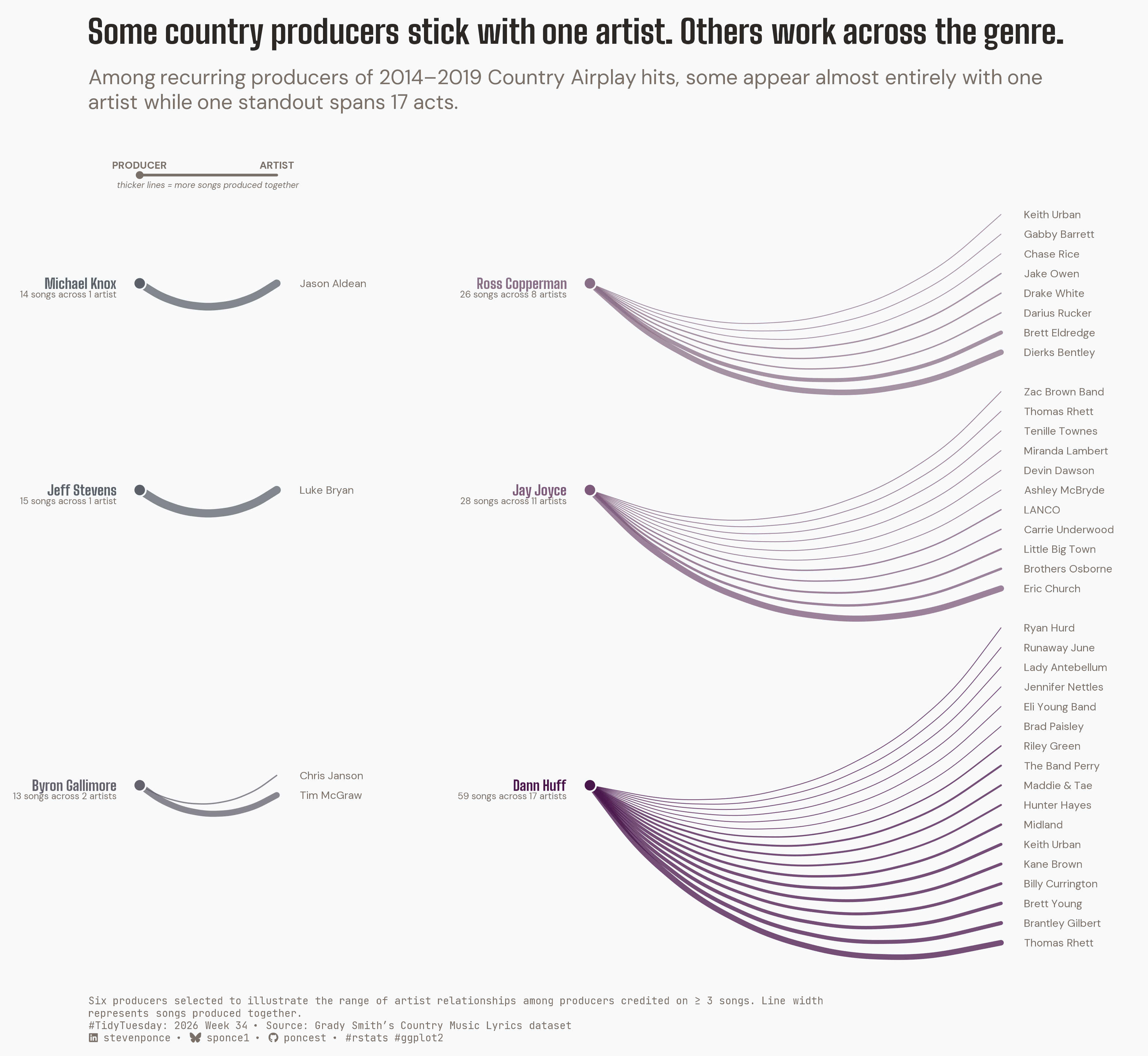
Among recurring producers of 2014–2019 Country Airplay hits, some appear almost entirely with one artist while one standout spans 17 acts.

An arc diagram comparing six country music producers’ artist relationships from 2014–2019 Country Airplay hits, where some work almost exclusively with one artist while Dann Huff spans 17 different acts. Producers were selected to illustrate this range from a larger set credited on three or more songs, with line width encoding songs produced together. Built in R with ggplot2.

Figure 1: Arc diagram titled “Some country producers stick with one artist. Others work across the genre.” Six country music producers are shown on the left, connected by curved lines to the artists they produced for during 2014-2019, with line width scaled to the number of songs produced together. Michael Knox and Jeff Stevens each connect to a single artist, Jason Aldean and Luke Bryan. Byron Gallimore mainly connects with Tim McGraw. Ross Copperman and Jay Joyce fan out to 8 and 11 artists respectively. Dann Huff, highlighted in burgundy, stands apart with 59 songs across 17 different artists, the widest network in the group. Producers were selected to illustrate this range from a larger set credited on three or more songs. Source: Grady Smith’s Country Music Lyrics dataset via TidyTuesday.

Steps to Create this Graphic

1. Load Packages & Setup

```{r}
#| label: load
#| warning: false
#| message: false      
#| results: "hide"     

## 1. LOAD PACKAGES & SETUP ----
suppressPackageStartupMessages({
if (!require("pacman")) install.packages("pacman")
pacman::p_load(
    tidyverse, ggtext, showtext, janitor, ggrepel,      
    scales, glue, skimr, ggview
    )
})

# Source utility functions
suppressMessages(source(here::here("R/utils/fonts.R")))
source(here::here("R/utils/social_icons.R"))
source(here::here("R/utils/image_utils.R"))
source(here::here("R/themes/base_theme.R"))
```

2. Read in the Data

```{r}
#| label: read
#| include: true
#| eval: true
#| warning: false

## 2. READ IN THE DATA ----
# tt <- tidytuesdayR::tt_load(2026, week = 34)
# country_lyrics <- tt$country_lyrics
# rm(tt)
country_lyrics <- readr::read_csv('https://raw.githubusercontent.com/rfordatascience/tidytuesday/main/data/2026/2026-08-25/country_lyrics.csv')
```

3. Examine the Data

```{r}
#| label: examine
#| include: true
#| eval: true
#| results: 'hide'
#| warning: false

## 3. EXAMINING THE DATA ----
glimpse(country_lyrics)
skim_without_charts(country_lyrics)
```

4. Tidy Data

```{r}
#| label: tidy
#| warning: false

hero_producers <- c(
  "Michael Knox",
  "Jeff Stevens",
  "Byron Gallimore",
  "Ross Copperman",
  "Jay Joyce",
  "Dann Huff"
)

producer_edges <- country_lyrics |>
  filter(!is.na(producer)) |>
  separate_longer_delim(producer, delim = ",") |>
  mutate(producer = str_squish(producer)) |>
  filter(producer %in% hero_producers) |>
  count(producer, artist, name = "n_songs")

#
producer_check <- producer_edges |>
  mutate(
    artist_share = n_songs / sum(n_songs),
    .by = producer
  ) |>
  summarise(
    total_songs = sum(n_songs),
    distinct_artists = n_distinct(artist),
    top_artist_share = max(artist_share),
    .by = producer
  ) |>
  arrange(match(producer, hero_producers))

# Two-column layout
reach_left <- 0.70
reach_right <- 2.10
col_gap <- 2.30
label_offset <- 0.12
row_gap <- 2.00

layout_spec <- tribble(
  ~producer, ~side, ~row,
  "Michael Knox", "left", 1,
  "Ross Copperman", "right", 1,
  "Jeff Stevens", "left", 2,
  "Jay Joyce", "right", 2,
  "Byron Gallimore", "left", 3,
  "Dann Huff", "right", 3
)

row_layout <- layout_spec |>
  left_join(producer_check, by = "producer") |>
  mutate(
    half_span = pmax((distinct_artists - 1) / 2, 0.5)
  ) |>
  summarise(
    row_half_span = max(half_span),
    .by = row
  ) |>
  arrange(row) |>
  mutate(
    row_full_span = row_half_span * 2,
    baseline_y = -(
      cumsum(row_full_span) -
        row_half_span +
        row_gap * (row_number() - 1)
    )
  ) |>
  select(row, row_half_span, baseline_y)

artist_breadth_range <- c(1, 17)
palette_fn <- scales::colour_ramp(c("#5C6068", "#90718A", "#4A154B"))

producer_layout <- layout_spec |>
  left_join(producer_check, by = "producer") |>
  left_join(row_layout, by = "row") |>
  mutate(
    half_span = pmax((distinct_artists - 1) / 2, 0.5),
    hub_x = if_else(
      side == "left",
      0,
      col_gap
    ),
    reach = if_else(
      side == "left",
      reach_left,
      reach_right
    ),
    node_x = hub_x + reach,
    producer_label_x = hub_x - label_offset,
    stat_label = str_glue(
      "{total_songs} songs across {distinct_artists} ",
      "{if_else(distinct_artists == 1, 'artist', 'artists')}"
    ),
    color_val = scales::rescale(
      distinct_artists,
      from = artist_breadth_range
    ),
    label_color = palette_fn(color_val)
  )

# Build artist nodes 
nodes <- producer_edges |>
  left_join(
    producer_layout |>
      select(
        producer,
        hub_x,
        node_x,
        baseline_y,
        distinct_artists
      ),
    by = "producer"
  ) |>
  mutate(
    producer = factor(
      producer,
      levels = layout_spec$producer
    )
  ) |>
  arrange(
    producer,
    desc(n_songs),
    artist
  ) |>
  mutate(
    rank = row_number(),
    k    = n(),
    .by  = producer
  ) |>
  mutate(
    y_local = rank - (k + 1) / 2,
    y_abs = baseline_y + y_local,
    artist_label_x = node_x + label_offset,
    color_val = scales::rescale(
      distinct_artists,
      from = artist_breadth_range
    ),
    line_color = palette_fn(color_val)
  )

# Visual Key

key_gap <- 2

key_y <- row_layout$baseline_y[row_layout$row == 1] +
  row_layout$row_half_span[row_layout$row == 1] +
  key_gap

key_data <- tibble(
  x    = 0,
  xend = reach_left,
  y    = key_y
)
```

5. Visualization Parameters

```{r}
#| label: params
#| include: true
#| warning: false

### |-  plot aesthetics ----
colors <- get_theme_colors()

bg_color <- "#F8F9FA"
title_color    <- colors$title
text_color     <- colors$text
subtitle_color <- colors$subtitle
caption_color  <- colors$caption

### |- titles and caption ----
title_text <- paste0(
  "Some country producers stick with one artist. ",
  "Others work across the genre."
)

subtitle_text <- paste0(
  "Among recurring producers of 2014\u20132019 Country Airplay hits, ",
  "some appear almost entirely with one artist while one standout spans 17 acts."
)

methodology_text <- str_wrap(
  paste0(
    "Six producers selected to illustrate the range of artist relationships ",
    "among producers credited on \u2265 3 songs. ",
    "Line width represents songs produced together."
  ),
  width = 130
) |>
  str_replace_all("\n", "<br>")

caption_text <- str_glue(
  "{methodology_text}<br>",
  "{create_social_caption(
      tt_year = 2026,
      tt_week = 34,
      source_text = \"Grady Smith's Country Music Lyrics dataset\"
    )}"
)

### |-  fonts ----
setup_fonts()
fonts <- get_font_families()
```

6. Plot

```{r}
#| label: plot
#| warning: false

### |-  plot ----
p <- ggplot(nodes) +
  # Producer - artist relationships
  geom_curve(
    aes(
      x = hub_x, y = baseline_y, xend = node_x, yend = y_abs,
      linewidth = n_songs, color = line_color
    ),
    curvature = 0.35, alpha = 0.75, lineend = "round"
  ) +
  geom_point(
    data = producer_layout,
    aes(x = hub_x, y = baseline_y),
    color = bg_color, size = 4.5
  ) +
  # Producer origin nodes
  geom_point(
    data = producer_layout,
    aes(x = hub_x, y = baseline_y, color = label_color), size = 3.2
  ) +
  # Artist labels
  geom_text(
    aes(x = artist_label_x, y = y_abs, label = artist),
    hjust = 0, size = 2.8, color = text_color, family = fonts$text
  ) +
  # Producer labels
  geom_text(
    data = producer_layout,
    aes(x = producer_label_x, y = baseline_y, label = producer, color = label_color),
    hjust = 1, fontface = "bold", size = 3.6, family = fonts$title_2
  ) +
  # Producer summary labels
  geom_text(
    data = producer_layout,
    aes(x = producer_label_x, y = baseline_y - 0.55, label = stat_label),
    hjust = 1, size = 2.4, color = text_color, family = fonts$text
  ) +
  # Visual key
  geom_segment(
    data = key_data,
    aes(x = x, y = y, xend = xend, yend = y),
    linewidth = 1, color = text_color, lineend = "round"
  ) +
  geom_point(
    data = key_data,
    aes(x = x, y = y),
    size = 2.2, color = text_color
  ) +
  geom_text(
    data = key_data,
    aes(x = x, y = y + 0.5, label = "PRODUCER"),
    hjust = 0.5, size = 2.6, fontface = "bold",
    color = text_color, family = fonts$text
  ) +
  geom_text(
    data = key_data,
    aes(x = xend, y = y + 0.5, label = "ARTIST"),
    hjust = 0.5, size = 2.6, fontface = "bold",
    color = text_color, family = fonts$text
  ) +
  geom_text(
    data = key_data,
    aes(
      x = (x + xend) / 2, y = y - 0.5,
      label = "thicker lines = more songs produced together"
    ),
    hjust = 0.5, size = 2.2, fontface = "italic",
    color = text_color, family = fonts$text
  ) +
  scale_linewidth_continuous(range = c(0.3, 3), guide = "none") +
  scale_color_identity() +
  scale_x_continuous(expand = expansion(mult = c(0.03, 0.08))) +
  coord_cartesian(clip = "off") +
  labs(
    title = title_text,
    subtitle = subtitle_text,
    caption = caption_text
  ) +
  theme_void() +
  theme(
    plot.background = element_rect(fill = bg_color, color = bg_color),
    panel.background = element_rect(fill = bg_color, color = bg_color),
    plot.title = element_textbox_simple(
      face = "bold", family = fonts$title_1, size = 24,
      lineheight = 1.2, color = title_color, margin = margin(b = 10)
    ),
    plot.subtitle = element_textbox_simple(
      family = fonts$subtitle, size = 15, lineheight = 1.3,
      color = subtitle_color, margin = margin(t = 5, b = 10)
    ),
    plot.caption = element_textbox_simple(
      family = fonts$caption, size = 7.5, color = caption_color,
      lineheight = 1.3, margin = margin(t = 12)
    ),
    plot.margin = margin(t = 14, r = 40, b = 10, l = 70)
  )
```

7. Save

```{r}
#| label: save
#| warning: false

### |- save ----
main_path  <- here::here("data_visualizations", "TidyTuesday", "2026", "tt_2026_34.png")
thumb_path <- here::here("data_visualizations", "TidyTuesday", "2026", "thumbnails", "tt_2026_34.png")

# Full-size version, for the QMD figure
save_ggplot(
  plot = p,
  file = main_path,
  width = 12.5,
  height = 11.5,
  units = "in",
  dpi = 300,
  create.dir = TRUE
)

# Reduced-size thumbnail, for the YAML `image:` field
fs::dir_create(dirname(thumb_path))
magick::image_read(main_path) |>
  magick::image_resize("400") |>
  magick::image_write(thumb_path)
```

8. Session Info

TipExpand for Session Info

R version 4.6.1 (2026-06-24)
Platform: aarch64-apple-darwin23
Running under: macOS Tahoe 26.5.2

Matrix products: default
BLAS:   /Library/Frameworks/R.framework/Versions/4.6/Resources/lib/libRblas.0.dylib 
LAPACK: /Library/Frameworks/R.framework/Versions/4.6/Resources/lib/libRlapack.dylib;  LAPACK version 3.12.1

locale:
[1] en_US.UTF-8/en_US.UTF-8/en_US.UTF-8/C/en_US.UTF-8/en_US.UTF-8

time zone: America/New_York
tzcode source: internal

attached base packages:
[1] stats     graphics  grDevices utils     datasets  methods   base     

other attached packages:
 [1] here_1.0.2      ggview_0.2.2    skimr_2.2.2     glue_1.8.1     
 [5] scales_1.4.0    ggrepel_0.9.8   janitor_2.2.1   showtext_0.9-8 
 [9] showtextdb_3.0  sysfonts_0.8.9  ggtext_0.1.2    lubridate_1.9.5
[13] forcats_1.0.1   stringr_1.6.0   dplyr_1.2.1     purrr_1.2.2    
[17] readr_2.2.0     tidyr_1.3.2     tibble_3.3.1    ggplot2_4.0.3  
[21] tidyverse_2.0.0 pacman_0.5.1   

loaded via a namespace (and not attached):
 [1] gtable_0.3.6       xfun_0.60          htmlwidgets_1.6.4  tzdb_0.5.0        
 [5] vctrs_0.7.3        tools_4.6.1        generics_0.1.4     curl_7.1.0        
 [9] parallel_4.6.1     pkgconfig_2.0.3    RColorBrewer_1.1-3 S7_0.2.2          
[13] lifecycle_1.0.5    compiler_4.6.1     farver_2.1.2       textshaping_1.0.5 
[17] repr_1.1.7         codetools_0.2-20   snakecase_0.11.1   litedown_0.10     
[21] htmltools_0.5.9    yaml_2.3.12        pillar_1.11.1      crayon_1.5.3      
[25] magick_2.9.1       commonmark_2.0.0   tidyselect_1.2.1   digest_0.6.39     
[29] stringi_1.8.7      labeling_0.4.3     rprojroot_2.1.1    fastmap_1.2.0     
[33] grid_4.6.1         cli_3.6.6          magrittr_2.0.5     base64enc_0.1-6   
[37] withr_3.0.3        bit64_4.8.2        timechange_0.4.0   rmarkdown_2.31    
[41] bit_4.6.0          otel_0.2.0         ragg_1.5.2         hms_1.1.4         
[45] evaluate_1.0.5     knitr_1.51         markdown_2.0       rlang_1.3.0       
[49] gridtext_0.1.6     Rcpp_1.1.2         xml2_1.6.0         rstudioapi_0.19.0 
[53] vroom_1.7.1        jsonlite_2.0.0     R6_2.6.1           fs_2.1.0          
[57] systemfonts_1.3.2 

9. GitHub Repository

TipExpand for GitHub Repo

The complete code for this analysis is available in tt_2026_34.qmd.

For the full repository, click here.

10. References

TipExpand for References

1. Data Source:
   • TidyTuesday 2026 Week 34: Country Music Lyrics

11. Custom Functions Documentation

Note📦 Custom Helper Functions

This analysis uses custom functions from my personal module library for efficiency and consistency across projects.

Functions Used:

• fonts.R: setup_fonts(), get_font_families() - Font management with showtext
• social_icons.R: create_social_caption() - Generates formatted social media captions
• image_utils.R: save_plot() - Consistent plot saving with naming conventions
• base_theme.R: create_base_theme(), extend_weekly_theme(), get_theme_colors() - Custom ggplot2 themes

Why custom functions?
These utilities standardize theming, fonts, and output across all my data visualizations. The core analysis (data tidying and visualization logic) uses only standard tidyverse packages.

Source Code:
View all custom functions → GitHub: R/utils